Abstract
Paper 1107 counted, through the singular values of kernel matrices, that when a field obeys a local equation of second order, what can be read from outside a closed skin is one number per angular pattern, two for fourth order and three for sixth order. This paper carries the same counting over into the language of statistics. In a Gaussian random field (a field whose values jointly follow a multivariate normal distribution), a zero in the precision matrix, the inverse of the covariance, means that two points are independent once all the others are known. The set of points that must be known to make a set of points independent of everything else is called its Markov blanket (Pearl 1988). When the precision matrix is built from the lattice Laplacian L as (κ² + L) to the power k (a local equation of order 2k), the blanket is exactly k layers thick. This is checked numerically and shown to be the same number as in Paper 1107. This paper claims no new theorem or law.
The nonzero entries in a row of the precision matrix are exactly the points within path distance k on the lattice: for k = 1, 2, 3 there are 5, 13, 25 of them in two dimensions and 7, 25, 63 in three. When m layers around a 3×3 block in a two-dimensional lattice are known, the conditional correlation between the block and the rest is exactly 0 for m at least k (0 in the computation as well), and remains when one layer is missing (0.159311 when only one layer is known for k = 2, and 0.070604 when only two layers are known for k = 3).
The number of ways in which the inside and the outside communicate was counted as the number of canonical correlations (Hotelling 1936). On a one-dimensional chain it is k, and the next value falls to the size of the numerical error (at most 7.50×10⁻¹⁶ of the largest). On a cylinder with 12 points in the periodic direction it is 12k, exactly k for each pattern in the periodic direction. Reading the kernels of Paper 1107 as covariances and counting, on the same grid with the same threshold, the singular values of the same inside–outside covariance as in Paper 1107, exp(−d)/d, exp(−d), (1+d)exp(−d) and (1+d+d²/3)exp(−d) in three dimensions stop at 1, 2, 3 and 4 per angular pattern. These kernels are the Green functions of the equations obtained by applying (κ² − Δ) once, twice, three and four times (checked symbolically). For kernels that stop, this count is the rank of the matrix and equals the number of canonical correlations. The Gaussian exp(−d²) does not stop, and the count cut by the threshold is 7, 7, 6, 6, 6, the same as in Paper 1107 (the same matrix built with a different quadrature). Its canonical correlations line up close to 1 and are a different thing from this count. The same covariance exp(−r) stops at 1 in one dimension and at 2 in three dimensions, but does not stop in two. Its Fourier transform is inversely proportional to (1 + ω²) to the power (d + 1)/2, and only in two dimensions is that power not an integer.
The thickness of the blanket is distinct from how far correlation reaches. With κ² = 0.01 in two dimensions, the correlation with a point 10 away is 0.118195, yet once the neighbouring layer is known the central point stays independent of the rest. The mutual information between a block of side L and the rest grows by almost 0.1939 per unit of side in two dimensions and nearly in proportion to L² in three (an area law; the log-log slopes are 1.0116 and 2.0210), and the slope does not change when k goes from 1 to 2. The area law itself appears even without a blanket (the lowest state of Paper 1107). That a blanket exists comes from the locality of the interaction, and its thickness from the order of the equation, splitting in the same way as the roots of Paper 1107. The debate on describing the boundary of living things by Markov blankets is not entered; only what has the same form is laid side by side. The separator is the order of the local equation that the precision matrix is.
Keywords: Markov blanket, Gaussian Markov random field, precision matrix, conditional independence, canonical correlation, order of the equation, area law, separator.
Scope (what is not claimed)
This paper claims no new theorem or law. The idea of a Markov blanket (Pearl 1988), that a zero in the precision matrix of a Gaussian random field means independence conditional on all the others (Besag 1974, Rue and Held 2005), that the Green functions of powers of (κ² − Δ) give covariances of Matérn type whose precision is local when the power is an integer (Whittle 1954, Lindgren, Rue and Lindström 2011), that a stationary Gaussian field has a blanket of finite thickness when its spectral density is the reciprocal of a polynomial (cited in connection with Rozanov 1982; the original has not been read), canonical correlations (Hotelling 1936), that the number of canonical correlations between past and future equals the dimension of the state (Akaike 1975), and that in warm states of local interactions the mutual information between a part and the rest grows with the size of the boundary (Wolf et al. 2008) are all known. That the zero pattern of a lattice precision matrix gives a blanket of k layers, and that a continuous-time autoregression sampled at equally spaced points does not stay an autoregression on the points, also appear to be standard computations in spatial statistics and time-series analysis. What is added is reading the kernels as covariances with the same kernels, the same grid and the same threshold with which Paper 1107 counted the numbers leaving the skin, and lining up that for kernels that stop the count equals the number of canonical correlations, the thickness of the blanket and half the order of the equation (and that for kernels that do not stop the two differ); checking on a cylinder that it is k for each pattern in the periodic direction; placing in one table that the same exponential covariance exp(−r) stops in one and three dimensions but not in two; lining up on the same chain, for a continuous covariance sampled at lattice points, the number of canonical correlations and the fact that knowing all the points in between does not separate the two sides; laying out in numbers, together with the size of the correlations, that the thickness does not depend on the reach of correlation (which follows from κ not entering the zero pattern), and placing it in the same form as the mass of the field in Paper 1107, which did not change the number leaving; and laying the area law onto the split of roots in Paper 1107. Whether this arrangement has precedents in the literature is left open. The free energy principle (Friston 2013) describes the boundary of living things by Markov blankets, and that use is debated (Bruineberg et al. 2022). This paper does not enter the debate, and says neither that cell membranes or brains are Markov blankets nor that they are not. It says only that, on a model whose fluctuations are Gaussian and whose precision comes from a local equation, the thickness of the blanket is half the order of the equation. The merits of methods that infer the zero pattern of a precision matrix from data (Friedman, Hastie and Tibshirani 2008) are not treated either. Non-Gaussian fields, blankets in graphs with arrows (Bayesian networks), and entanglement of quantum fields are not treated. Paper 1107 counted that the numbers readable from outside a closed skin are, per angular pattern, half the order of the equation, and separated as distinct roots that one skin suffices (second order), that 4π remains on the skin (a massless field), and the area law (locality of the interaction). This paper sits beside it and reads the same kernels as covariances. Paper 1051 wrote whether the boundary determines the interior in terms of what is measured and how much. The blanket of this paper is the answer to what, and how much, must be known on the boundary to cut the inside off from the outside. The Gauss–Markov theorem treated in Paper 171 (among linear unbiased estimators, least squares has the smallest variance) has a similar name but is a different matter from the blanket here.
1. Numbers leaving the skin, and the thickness of the blanket
Paper 1107 counted, through the singular values of the kernel matrix from inner radii to outer radii, how many numbers leave a closed skin per angular pattern (each spherical harmonic) when the source inside is read only from the field outside the skin. The inverse-square kernel $1/r$ and the Yukawa kernel $e^{-r}/r$ in three dimensions give 1 per pattern, the biharmonic kernel 2 and the triharmonic kernel 3, while power kernels and the Gaussian kernel do not stop. The kernels that stop are fundamental solutions of local equations whose form does not change under rotation, and the number leaving the skin was half the order of that equation.
Statistics has a question of the same form. When many quantities are correlated with one another, what around a block must be known to cut it off from everything else? For a Gaussian random field, that is, a field whose values jointly follow a multivariate normal distribution, the answer is written with one matrix. Take the mean to be 0 and the covariance to be $\Sigma$, and call its inverse $Q=\Sigma^{-1}$ the precision matrix. Two points $i$ and $j$ are independent once all other points are known if and only if $Q_{ij}=0$ (Besag 1974, Rue and Held 2005). For a set of points $A$, a set of points that, once known, makes $A$ independent of everything else is called a Markov blanket, and Pearl called the smallest such set the Markov boundary (Pearl 1988). In this paper the set of outer points that $Q$ connects to $A$ (this smallest set) is called the blanket of $A$. Once the blanket is known, $A$ is independent of everything else.
This paper counts the thickness of the blanket when the precision matrix comes from a local equation. The lattice spacing is 1, and with the lattice Laplacian written $L$ (the matrix with $2d$ on the diagonal and $-1$ for neighbours, $d$ being the dimension),
$$Q=(\kappa^2 I+L)^k,\qquad k=1,2,3.$$This is $(\kappa^2-\Delta)^k$ of a continuous field moved onto the lattice, a local equation of order $2k$. Here $\kappa$ corresponds to the mass of a Yukawa field, and correlation reaches a distance of order $1/\kappa$. The covariance $\Sigma=Q^{-1}$ is the Green function of this equation. Unless stated otherwise, $\kappa^2=0.5$. Inverses and singular values were computed in double precision (the comparison with canonical correlations in Section 5 in 80 digits), Green functions were checked symbolically (in two dimensions by 40-digit values), and Fourier transforms by 30-digit quadrature.
2. The zero pattern of the precision matrix
Since $L$ connects only neighbours, $Q$, which multiplies $L$ $k$ times, connects only points reachable within $k$ steps on the lattice. With $\kappa^2=1$, $Q$ was built in integers and the nonzero entries in a row were counted (the lattice is periodic).
| dimension | $k=1$ | $k=2$ | $k=3$ | formula (number of points within path distance $k$) |
|---|---|---|---|---|
| 1 | 3 | 5 | 7 | $2k+1$ |
| 2 | 5 | 13 | 25 | $2k^2+2k+1$ |
| 3 | 7 | 25 | 63 | $(2k+1)(2k^2+2k+3)/3$ |
The nonzero entries were exactly the points whose path distance on the lattice (the sum of the absolute differences of the coordinates) is at most $k$, for every row in one and two dimensions and for one row in three. The count is the number of lattice points within path distance $k$ itself. With $\kappa^2=0.5$ the pattern does not change. The infinite lattice can be coloured with two colours (on a periodic lattice with at least $2k+1$ points per side the same holds within $k$ steps), so every walk joining two points has the parity of their distance. When $(\kappa^2I+L)^k$ is expanded in powers of the adjacency matrix, every term therefore carries the sign of $-1$ raised to the distance, and the terms do not cancel (for any $\kappa^2\geq0$). That the sign of each nonzero entry is exactly $-1$ raised to the distance was also checked for $\kappa^2=1$ and 0.5.
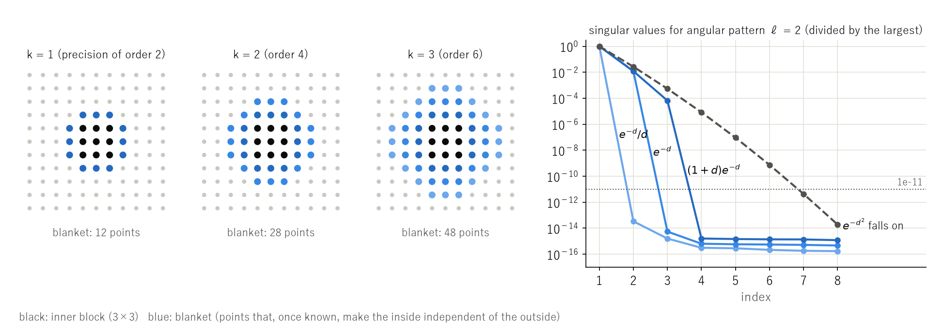
The blanket of a set of points $A$ is therefore the set of points at path distance 1 to $k$ from $A$, $k$ layers thick. For a $3\times3$ block in two dimensions the layers at distances 1, 2, 3 have 12, 16, 20 points, and the blanket has 12, 28, 48 points for $k=1$, 2, 3. For one point in three dimensions the layers have 6, 18, 38 points and the blanket 6, 24, 62 (Fig. 1 left). In every case this agreed with the set counted as the outer points that $Q$ connects to the block.
3. One layer short, the outside leaks in
That knowing the blanket makes the inside independent of the outside is checked by conditional correlations. A $3\times3$ block $A$ is placed at the centre of a periodic two-dimensional lattice ($21\times21$), and the layers at distance 1 to $m$ from the block are taken as known. What is unknown is the block and the rest $B$ at distance greater than $m$. Given the layers, the covariance of $(A,B)$ is the inverse of $Q$ restricted to the points of $A$ and $B$; the largest of its $A$–$B$ entries divided by the respective standard deviations (the conditional correlation) and the conditional mutual information (in nats) are listed. $m=0$ is the case where nothing is known: the ordinary correlation and mutual information between the block and the rest. Each cell reads "correlation / information".
| layers known | $k=1$ (order 2) | $k=2$ (order 4) | $k=3$ (order 6) |
|---|---|---|---|
| $m=0$ (nothing known) | 0.3344 / 0.5630 | 0.6797 / 2.2534 | 0.8647 / 5.0897 |
| $m=1$ | 0 / 0 | 0.1593 / 0.1012 | 0.3888 / 0.6213 |
| $m=2$ | 0 / 0 | 0 / 0 | 0.0706 / 0.0202 |
| $m=3$ | 0 / 0 | 0 / 0 | 0 / 0 |
For $m$ at least $k$, both correlation and information are exactly 0, and 0 in the computation as well: once the layers are known, $Q$ splits into a part for $A$ and a part for $B$, and so does its inverse. One layer short, at $m=k-1$, a correlation of 0.159311 remains for $k=2$ and 0.070604 for $k=3$. The same holds at the central point of a periodic three-dimensional lattice ($11\times11\times11$): 0 for $m\geq k$, and one layer short 0.0748 remains for $k=2$ and 0.0269 for $k=3$. In a field obeying a fourth-order equation, even when the neighbouring layer is known, word from points two steps away jumps over that layer and arrives.
4. The number of ways inside and outside communicate
What Paper 1107 counted was how many numbers are carried from the source inside to the field outside. Its counterpart in statistics is the number of canonical correlations (Hotelling 1936) between the quantities inside and outside. With covariances $\Sigma_{AA}$, $\Sigma_{BB}$ and $\Sigma_{AB}$ for the inner set $x_A$ and the outer set $x_B$, the canonical correlations are the singular values of $\Sigma_{AA}^{-1/2}\Sigma_{AB}\Sigma_{BB}^{-1/2}$, the strengths of the mutually independent combinations through which inside and outside communicate. The number of nonzero canonical correlations equals the rank of $\Sigma_{AB}$. If a blanket $S$ separates $A$ and $B$, then $\Sigma_{AB}=\Sigma_{AS}\Sigma_{SS}^{-1}\Sigma_{SB}$, so the number does not exceed the number of points in the blanket. Values above $10^{-11}$ of the largest were counted (the same threshold as Paper 1107).
On a one-dimensional chain (64 points, open ends), the canonical correlations between the left 30 points and the right 30 points (4 points between) were counted. For $k=1$ there is one, $3.125\times10^{-2}$, followed by the size of the numerical error ($9.39\times10^{-20}$). This value agrees with $1/32=(1/2)^5$ within double-precision rounding (a difference of $3.47\times10^{-18}$): it is the smaller root $\rho=1/2$ of $\rho+1/\rho=2+\kappa^2=2.5$, multiplied over the 5 steps that separate left from right. For $k=2$ there are two, $1.42\times10^{-1}$ and $1.72\times10^{-3}$; for $k=3$ three, $3.48\times10^{-1}$, $1.23\times10^{-2}$ and $1.12\times10^{-4}$; and in every case the next falls to the size of the numerical error (at most $7.50\times10^{-16}$ of the largest). On a chain the blanket separating left from right is $k$ points, and the count equals that number of points.
To give the field something that plays the role of angular patterns, a cylinder ($40\times12$) with one direction periodic with 12 points was also used. The canonical correlations between the left 18 columns and the right 18 columns (4 columns between) number 12, 24, 36 for $k=1$, 2, 3, and the next is at the size of the numerical error (at most $1.30\times10^{-15}$ of the largest). Split into the 12 patterns of the periodic direction (constant, cosines and sines), every pattern has exactly $k$. The "half the order per pattern" of Paper 1107 appears here as "the number of layers of the blanket per pattern".
The count also stops when a covariance of a continuous field is sampled at integer points. With $t$ half the distance, chains whose covariance is $e^{-t}$, $(1+t)e^{-t}$ or $(1+t+t^2/3)e^{-t}$ have 1, 2, 3 canonical correlations, and the next value falls to the size of the numerical error (at most $3.86\times10^{-14}$ of the largest). These have the form of the Green functions of the equations obtained by applying $(\kappa^2-d^2/dx^2)$ once, twice and three times in one dimension. The inverse of the covariance $(1+t)e^{-t}$ sampled at integer points, however, is not banded: one row divided by its diagonal goes on as $7.25\times10^{-1}$, $2.86\times10^{-1}$ and $7.45\times10^{-2}$ at distances 1, 2, 3 (for $e^{-t}$ everything from distance 2 on is at the size of the numerical error, at most $1.35\times10^{-16}$). The blanket of the continuous field is the two numbers of value and slope at the boundary point, and lattice values cannot stand in for them even when all the points in between are known. With all 4 points in between known, the largest conditional correlation between left and right that remains is 0.00922 for $(1+t)e^{-t}$ and 0.0877 for $(1+t+t^2/3)e^{-t}$ (for $e^{-t}$ it is at the size of the numerical error). The number of ways of communicating stays 2, but what carries them is no longer a lattice layer.
Some covariances do not stop. The canonical correlations of the Gaussian $e^{-t^2}$ go $1.10\times10^{-2}$, $2.33\times10^{-5}$, $1.41\times10^{-8}$, $2.23\times10^{-12}$, $8.60\times10^{-17}$, falling by ratios of $3.86\times10^{-5}$ to $2.11\times10^{-3}$ per step, and those of the Cauchy form $1/(1+t^2)$ go $1.51\times10^{-1}$, $1.92\times10^{-2}$, $3.07\times10^{-3}$, $3.86\times10^{-4}$ and on down to $1.14\times10^{-7}$, falling by ratios of 0.0413 to 0.1598 per step. For the covariances that stop, the value after the last kept one drops at once to the size of the numerical error; these two keep falling step by step, and where to cut is decided by the threshold.
5. Reading the kernels of Paper 1107 as covariances
The kernels of Paper 1107 are read as covariances of a Gaussian field. The inner radius $s$ was taken from 0.05 to 0.8 and the outer radius $r$ from 1.25 to 3.0 at 40 points each, the pattern-$\ell$ component $K_\ell(r,s)$ (the formula of Paper 1107) was built by 400-point Gaussian quadrature in three dimensions and an 800-point equally spaced sum in two, and singular values above $10^{-11}$ of the largest were counted. Read as a covariance, $K_\ell(r,s)$ is the covariance between the pattern-$\ell$ quantity on the sphere of radius $s$ and the same pattern on the sphere of radius $r$. What was counted is the singular values of this inside–outside covariance $K_\ell(r,s)$, the same matrix as in Paper 1107, not the canonical correlations of Section 4 (which are divided by the inside–inside and outside–outside covariances). For kernels that stop, the number of nonzero singular values (the rank of the matrix) does not change under that division, so it equals the number of nonzero canonical correlations and is the number of ways the inside and the outside communicate. For kernels that do not stop, the count cut by the threshold is a different thing from the number of canonical correlations (laid out below). The biharmonic kernel $r$ of Paper 1107 is 0 at 0 and positive away from it, so it is not a covariance as it stands; as a covariance of the same fourth order but coming from $(\kappa^2-\Delta)^2$, $e^{-d}$ was used.
| dimension | covariance (kernel) | equation of the precision | count for patterns $\ell=0$ to 4 |
|---|---|---|---|
| 3 | $e^{-\kappa d}/d$ ($\kappa=0.1$, 1, 3) | $\kappa^2-\Delta$ (order 2) | 1, 1, 1, 1, 1 |
| 3 | $e^{-d}$, $e^{-2d}$ | $(\kappa^2-\Delta)^2$ (order 4) | 2, 2, 2, 2, 2 |
| 3 | $(1+d)e^{-d}$ | $(1-\Delta)^3$ (order 6) | 3, 3, 3, 3, 3 |
| 3 | $(1+d+d^2/3)e^{-d}$ | $(1-\Delta)^4$ (order 8) | 4, 4, 4, 4, 4 |
| 3 | $e^{-d^2}$ | none (Gaussian) | 7, 7, 6, 6, 6 (set by the threshold) |
| 2 | $K_0(d)$ | $1-\Delta$ (order 2) | 1, 1, 1, 1, 1 |
| 2 | $dK_1(d)$ | $(1-\Delta)^2$ (order 4) | 2, 2, 2, 2, 2 |
| 2 | $d^2K_2(d)$ | $(1-\Delta)^3$ (order 6) | 3, 3, 3, 3, 3 |
| 2 | $e^{-d}$ | none | 6, 6, 6, 6, 6 (set by the threshold) |
| 2 | $e^{-d^2}$ | none (Gaussian) | 7, 7, 6, 6, 6 (set by the threshold) |
| 1 | $e^{-|d|}$ | $1-d^2/dx^2$ (order 2) | 1, 1 (even, odd) |
| 1 | $(1+|d|)e^{-|d|}$ | $(1-d^2/dx^2)^2$ (order 4) | 2, 2 (even, odd) |
For the three-dimensional kernels that stop, the smallest kept value is $3.29\times10^{-8}$, while the next value stays at the size of the numerical error (at most $3.38\times10^{-12}$), a gap of about 4 orders of magnitude ($10^{3.99}$). This $3.38\times10^{-12}$ belongs to the Yukawa kernel with $\kappa=0.1$ and lies at 1/2.96 of the threshold (the counting follows Paper 1107, and the threshold was not changed). The 7, 7, 6, 6, 6 of the Gaussian is a count set by the threshold in both three and two dimensions. That the three-dimensional 7, 7, 6, 6, 6 is the same as in the table of Paper 1107 is because the same matrix, with the same kernel, the same radii and the same threshold, was built with a different quadrature.
For kernels that do not stop, the count cut by the threshold and the number of canonical correlations are different things. Laid out with few radii (8 inner and 8 outer points, pattern $\ell=0$, closed forms, 80 digits), the canonical correlations of the three-dimensional Gaussian $e^{-d^2}$ are 1.0, 1.0, 1.0, 0.99997, 0.989, 0.624, 0.0765, 0.00218: for a smooth field the quantities outside are almost fixed by those inside, and combinations close to 1 line up. The singular values of the inside–outside covariance with the same setting, divided by the largest, fall as 1, 0.0542, 0.00162, $3.25\times10^{-5}$, and the eighth is $1.42\times10^{-14}$. For $e^{-d}$, which stops, the canonical correlations 0.966, 0.236 and the singular values 1, 0.0108 are followed in both cases by values below $10^{-77}$, and both give 2.
That the kernels which stop come from the equations of the table was checked. In three dimensions,
$$G_1=\frac{e^{-\kappa r}}{4\pi r},\quad G_2=\frac{e^{-\kappa r}}{8\pi\kappa},\quad G_3=\frac{(1+\kappa r)e^{-\kappa r}}{32\pi\kappa^3},\quad G_4=\frac{(1+\kappa r+\kappa^2r^2/3)e^{-\kappa r}}{64\pi\kappa^5}$$satisfy $(\kappa^2-\Delta)G_{j+1}=G_j$ ($r>0$), $(\kappa^2-\Delta)G_1=0$, and $G_1$ sends a flux of 1 out of the origin (symbolic computation). So $G_j$ is the Green function of $(\kappa^2-\Delta)^j$, and the exponential covariance $e^{-d}$ comes from a fourth-order equation and $(1+d)e^{-d}$ from a sixth-order one. In two dimensions $K_0(\kappa r)/(2\pi)$, $rK_1(\kappa r)/(4\pi\kappa)$ and $r^2K_2(\kappa r)/(16\pi\kappa^2)$ satisfy the same relation (the remainder is below $10^{-25}$ in 40-digit computation), and in one dimension $e^{-\kappa|x|}/(2\kappa)$ and $(1+\kappa|x|)e^{-\kappa|x|}/(4\kappa^3)$ do.
The same $e^{-d}$ behaves differently with dimension. It stops at 1 in one dimension and at 2 in three, and does not stop in two (Fig. 1 right is three-dimensional). The singular values for pattern $\ell=2$ are 1 and $1.20\times10^{-2}$ followed by $5.52\times10^{-15}$ in three dimensions, but in two dimensions they go 1, $7.29\times10^{-3}$, $3.47\times10^{-5}$, $3.68\times10^{-7}$, $5.07\times10^{-9}$, $7.92\times10^{-11}$, falling on by ratios of $4.76\times10^{-3}$ to $1.56\times10^{-2}$ per step. The reason shows in the Fourier transform. The Fourier transform of $e^{-r}$ in $d$ dimensions is $2/(1+\omega^2)$ in one dimension, $2\pi/(1+\omega^2)^{3/2}$ in two and $8\pi/(1+\omega^2)^2$ in three (30-digit quadrature, within $10^{-20}$ at three values of $\omega$). If its reciprocal is a polynomial in $\omega^2$, the precision is the local equation $(1-\Delta)^{(d+1)/2}$, and the power is an integer only when $d$ is odd. That a stationary Gaussian field has a blanket of finite thickness when its spectral density is the reciprocal of a polynomial is cited in connection with Rozanov 1982 (see the scope note). For a covariance of Matérn type (with a smoothness number $\nu$), the question is whether $\nu+d/2$ is an integer (Whittle 1954, Lindgren et al. 2011). For $e^{-r}$, $\nu=1/2$ and $\nu+d/2$ is 1 in one dimension, $3/2$ in two and 2 in three. The kernels of the table that stop and those that do not split exactly as this criterion says.
6. The thickness does not depend on how far correlation reaches
$\kappa$ fixes how far correlation reaches but not the thickness of the blanket. On a periodic two-dimensional lattice ($41\times41$) with $k=1$, $\kappa^2$ was moved through 0.01, 0.25, 1 and 4. The correlation between the central point and a point 10 away moves widely, 0.118195, 0.001623, 0.000016 and $6.40\times10^{-9}$. Still, for every $\kappa$, once the 4 neighbours are known the central point is independent of all the rest (the conditional correlation is 0 in the computation). The variance of the central point is 0.649041, 0.376855, 0.254050, 0.134148, and knowing the 4 neighbours shrinks it to $1/(4+\kappa^2)$, that is 0.249377, 0.235294, 0.200000, 0.125000.
In Paper 1107 the mass $\kappa$ of the field decided whether the flux through the skin is $4\pi$ at every radius, but did not change how many numbers leave (the Yukawa kernel also gives 1 per pattern). Here too $\kappa$ fixes how far correlation reaches and does not change the thickness of the blanket. The three-dimensional $e^{-\kappa d}/d$ of the previous section also gave 1 per pattern for each of $\kappa=0.1$, 1, 3. However far the correlation reaches, it arrives only through a blanket one layer thick.
7. What grows with the size of the blanket
The mutual information between a block and the rest equals the mutual information between the block and its blanket, because once the blanket is known the block is independent of the rest. It should therefore grow with the size of the blanket, not with the number of points in the block. On periodic lattices, square and cubic blocks of side $L$ were taken and the mutual information $\frac12\log\det(\Sigma_{AA}Q_{AA})$ was computed ($Q_{AA}^{-1}$ is the covariance of the block given the rest).
In two dimensions ($24\times24$) with $k=1$ it grows from 0.3690 to 1.9205 for $L=2$ to 10, and the increase per unit of $L$ settles at 0.1939 from $L=6$ on. The slope of the last 4 points (log-log) is 1.0116: it grows as $L$ to the first power, that is, with the perimeter of the block. The slope is a little above 1 because the values for $L=6$ to 10 lie on the linear expression $0.19391L-0.01852$, whose intercept is negative (along this expression the log-log slope would come down to 1.0010 at $L=100$). In three dimensions ($12\times12\times12$) with $k=1$ it grows from 0.4753 to 4.3917 for $L=2$ to 6, with slope 2.0210, that is, with the surface area of the block (for $L=3$ to 6 the values differ from $0.12259L^2-0.02292$ by at most $1.61\times10^{-3}$ of themselves). With $k=2$ the increase per unit of $L$ in two dimensions becomes 0.7757, but the slope is 1.0118, and 2.0039 in three dimensions: the slope does not change.
This field is the same as the distribution of positions of the lattice springs $H=\frac12\sum_i(p_i^2+m_0^2x_i^2)+\frac12\sum_{\langle ij\rangle}(x_i-x_j)^2$ on which Paper 1107 checked the area law, placed at temperature 1 in classical statistics ($\kappa^2=m_0^2$, $k=1$). That in warm states of local interactions the mutual information between a part and the rest grows with the size of the boundary was shown by Wolf et al. 2008 (also cited in Paper 1107). The numbers of this section count that growth from the fact that, once the blanket is known, the block is independent of the rest. Paper 1107 placed the root of the area law in the locality of the interaction (finite reach), separate from the root of how many numbers leave (the order of the equation). Here too, that a blanket exists and the area law come from locality, and the thickness of the blanket from the order of the equation. The order changes the coefficient of the area law but not the slope.
The area law, however, appears even without a blanket. In the lowest state of the lattice springs of Paper 1107 the precision of the distribution of positions is $2(\kappa^2I+L)^{1/2}$, and one row divided by its diagonal only decreases along an axis, $1.23\times10^{-1}$, $9.04\times10^{-3}$, $1.54\times10^{-3}$, $3.67\times10^{-4}$ at distances 1, 2, 3, 4, without ending: there is no blanket of finite thickness. Still, on the same two-dimensional lattice ($24\times24$, $\kappa^2=0.5$) the mutual information of the positions alone grows from 0.0922 to 0.4802 for $L=2$ to 10, by almost 0.0485 per unit of side. A blanket is one road to the area law, and an area law does not imply a blanket.
8. A bridge to living things and machine learning
The language of Markov blankets is used outside statistics too. The free energy principle (Friston 2013) places, between the internal states of a living thing and the outside world, a Markov blanket made of sensory and active states, and uses it to describe the boundary of the living thing. This use has been criticised for not separating the blanket as a property of a statistical model from a claim about a real boundary (Bruineberg et al. 2022). What this paper counted is only the blanket of a given Gaussian model, and it says neither that cell membranes or brains are Markov blankets nor that they are not.
Only what has the same form is laid side by side. In a model whose fluctuations are Gaussian and whose precision comes from a local equation of order $2k$, the blanket has $k$ layers: one layer for a second-order equation such as diffusion, two for a fourth-order one such as bending. In the model that writes small fluctuations of the height of a membrane with a bending stiffness and a tension (the bending energy being that of Helfrich 1973), the precision is of fourth order, $\Delta^2$ plus $-\Delta$. Moving this form, which is not a perfect square, onto the lattice as $L^2+0.3L+0.05I$, the blanket is still exactly two layers (28 points), and knowing only one layer leaves a correlation of 0.2226 (the same lattice and block as Section 3).
In machine learning there is a way of inferring the zero pattern of the precision matrix (the graph of connections) from many quantities (Friedman, Hastie and Tibshirani 2008). Among prior distributions that impose smoothness, the one that penalises the square of second differences (the second-order random walk of Rue and Held 2005) corresponds to a fourth-order precision: one row is $6, -4, 1$ and ends at distance 2, and the blanket has two layers. The merits of the inference, and whether an inferred zero pattern is a real connection, are not treated.
9. Shared root or distinct roots
The quantities of this paper are sorted by the test of Paper 300.
(1) The numbers leaving the skin in Paper 1107 and the thickness of the blanket here (the number of ways inside and outside communicate): they share a root. For kernels that stop, a covariance is the Green function of the equation of the precision, and the very matrix whose singular values Paper 1107 counted becomes the covariance between inside and outside. The number of nonzero canonical correlations is the rank of this matrix, which does not change when it is divided by the inside–inside and outside–outside covariances. The two numbers are therefore not counted values that happen to agree but the same rank of the same matrix. That rank is the dimension of the state placed where inside and outside are separated (the statement of Akaike 1975 that the number of canonical correlations between past and future equals the dimension of the state, read for inside and outside), which on the lattice is the number of layers of the blanket, half the order of the equation. For the Gaussian kernel neither stops, but that the 7, 7, 6, 6, 6 cut by the threshold is the same as in Paper 1107 is because the same matrix was counted, and it is not counted as evidence of a shared root (counted by canonical correlations, values close to 1 line up).
(2) The thickness of the blanket and how far correlation reaches: distinct roots. Moving $\kappa$ moves the correlation with a point 10 away from 0.118195 to $6.40\times10^{-9}$, but the thickness stays one layer. This has the same form as in Paper 1107, where the mass of the field, which decided whether $4\pi$ remains on the skin, did not change how many numbers leave.
(3) That a blanket exists, and its thickness: distinct roots. That a blanket exists comes from the locality of the interaction, and the thickness from the order of the equation. Changing the order does not change the slope of the area law. The area law also comes from locality, but it appears even without a blanket (end of Section 7, the lowest state of Paper 1107).
(4) Lattice layers, and the value and slope at the boundary of a continuous field: as a number of ways of communicating they share a root, both being the dimension of the state placed where inside and outside are separated, which is 2 for $(1+t)e^{-t}$ and for the lattice with $k=2$ (Akaike 1975, read for inside and outside). As what carries them they are distinct. For the precision $(\kappa^2I+L)^k$ moved onto the lattice the state is the values at the layer points; for a continuous covariance sampled at points it is the value and slope at the boundary, which cannot be written with lattice values (knowing all 4 points in between still leaves a largest conditional correlation of 0.00922 between left and right).
10. The separator
The separator is the order of the local equation that the precision matrix is. For order $2k$ the blanket has $k$ layers, and the number of ways the inside and the outside communicate is $k$ per pattern, the same as the number leaving the skin in Paper 1107. For covariances that do not rest on a local equation (the Gaussian, the Cauchy form, $e^{-r}$ in two dimensions) the thickness of the blanket does not stop at a fixed number. $\kappa$ (how far correlation reaches) does not enter this separator. The separator of Paper 1107, the order of the local equation that the field obeys, serves as the separator on the side of statistics as well.
Closing
For a Gaussian field built on a local equation of order 2k, the Markov blanket is k layers thick, half the order of the equation. The zero pattern of the precision matrix stays within path distance k on the lattice, and removing one layer lets the outside leak in. The number of ways the inside and the outside communicate is k per angular pattern, the same number that Paper 1107 counted as the numbers leaving the skin (for kernels that stop, the same rank of the same matrix). Paper 1107 read the same kernels as the map from a source to the field outside, and this paper read them as covariances. How far correlation reaches does not change the thickness; that a blanket exists and the area law come from locality, and the thickness from the order of the equation.
References
- Akaike, H. (1975). Markovian representation of stochastic processes by canonical variables. SIAM Journal on Control.
- Besag, J. (1974). Spatial interaction and the statistical analysis of lattice systems. Journal of the Royal Statistical Society, Series B.
- Bruineberg, J., Dołęga, K., Dewhurst, J., and Baltieri, M. (2022). The Emperor’s New Markov Blankets. Behavioral and Brain Sciences.
- Friedman, J., Hastie, T., and Tibshirani, R. (2008). Sparse inverse covariance estimation with the graphical lasso. Biostatistics.
- Friston, K. (2013). Life as we know it. Journal of the Royal Society Interface.
- Helfrich, W. (1973). Elastic properties of lipid bilayers: theory and possible experiments. Zeitschrift für Naturforschung C.
- Hotelling, H. (1936). Relations between two sets of variates. Biometrika.
- Lindgren, F., Rue, H., and Lindström, J. (2011). An explicit link between Gaussian fields and Gaussian Markov random fields: the stochastic partial differential equation approach. Journal of the Royal Statistical Society, Series B.
- Pearl, J. (1988). Probabilistic Reasoning in Intelligent Systems: Networks of Plausible Inference. Morgan Kaufmann.
- Rozanov, Yu. A. (1982). Markov Random Fields. Springer.
- Rue, H. and Held, L. (2005). Gaussian Markov Random Fields: Theory and Applications. Chapman & Hall/CRC.
- Whittle, P. (1954). On stationary processes in the plane. Biometrika.
- Wolf, M. M., Verstraete, F., Hastings, M. B., and Cirac, J. I. (2008). Area laws in quantum systems: Mutual information and correlations. Physical Review Letters.
- Yamagishi, Y. (2026). The Fence around Least Squares Is Linearity, Not Normality [Paper 171]. YOI: https://www.yamagishiyuuki.com/yoi/171; DOI: 10.5281/zenodo.22094287
- Yamagishi, Y. (2026). The Three Hundredth Census: Whether Two Things Share a Root Is Decidable [Paper 300]. YOI: https://www.yamagishiyuuki.com/yoi/300; DOI: 10.5281/zenodo.22171914
- Yamagishi, Y. (2026). Whether the Boundary Determines the Interior Depends on What Is Measured and How Much [Paper 1051]. YOI: https://www.yamagishiyuuki.com/yoi/1051; DOI: 10.5281/zenodo.22903544
- Yamagishi, Y. (2026). When the Field Equation Is of Second Order, the Interior Can Be Read from Outside a Closed Skin Only as One Number per Angular Pattern [Paper 1107]. YOI: https://www.yamagishiyuuki.com/yoi/1107
Reference
Yamagishi, Y. (2026). For a Gaussian Field Built on a Local Equation, the Markov Blanket Is as Thick as Half the Order of That Equation [Paper 1122]. YOI: https://www.yamagishiyuuki.com/yoi/1122
ORCID: 0009-0006-8587-3450
PDF (English) · PDF (Japanese) · Date proof of the English PDF (OpenTimestamps .ots) · SHA256SUMS
The record page for this paper (in Japanese, with the PDFs in each language and the date proof): YOI 1122. This paper is a preprint and has not been peer reviewed.