PDF (a copy kept with this page, identical to the archived original): yamagishi_yoi1109_v1_en.pdf
Abstract
An atom with a full shell is perfectly round on average, and it sends no number (multipole) out through a closed skin. Yet noble gases turn liquid when cooled. With hydrogen and a spring model, this paper counts how the attraction comes not from the average shape but from the product of fluctuating lopsidedness. In the 1s state of hydrogen the average lopsidedness ⟨z⟩ is 0, but the mean square ⟨z²⟩ is ⟨r²⟩/3 = 1 (in units of the Bohr radius squared). In the solvable model of two charges bound by springs (ħ = m = ω0 = 1, polarizability α = 1), with coupling strength κ = α/R³ between the dipoles, the zero-point energy at zero temperature falls by (3/4)κ² (in units of ħω0) for small κ. At R = 10 the exact value divided by this formula is 1.000001, and the exponent from R = 10 to 20 is −6.000001. The average lopsidedness stays 0 while the two line up: at κ = 0.1 the correlation coefficient is 0.1010 along the joining line (same direction) and −0.0501 sideways (opposite directions). Solving the p rooms of hydrogen in a Laguerre-type basis of the same form as Mitroy and Bromley (2005) and retracing their sum over pseudo-states, the coefficient C6 between two hydrogen atoms is 6.4990267053304 with 10 basis functions (the same as the 10-function column of their table to 13 digits) and 6.4990267054 from 20 on, matching the best value of the table to 13 digits. London’s simple formula keeps the true polarizability 9/2 and puts only the excitation energy at the ionization energy I = 1/2, giving (3/4)Iα² = 7.593750, 1.168444 times the true value. Of the true polarizability, 0.657694 comes from the transition to 2p (ΔE = 3/8), below I, so the energy of a single line that matches C6 is 0.427919, below I, and the ratio 1.168444 is exactly I ÷ 0.427919.
Splitting the source of the fluctuation by temperature, the free energy falls by (3/4)κ²ħω0 through zero-point fluctuation when kT is far below ħω0, and by 3kTκ² through thermal fluctuation when kT is far above. The two approximate formulas cross at kT = ħω0/4, and the thermal addition equals the zero-point part at kT = 0.490228ħω0. The thermal attraction comes not from the internal energy but from the entropy term (at kT = 10, ΔU/κ² = −0.000017 and ΔF/κ² = −30.000049). If the ħω0 of an atom is of the size of a hartree, room-temperature kT is 0.000950 of it, and at distances short enough that delay does not matter the zero-point fluctuation wins. In d dimensions the dipole field weakens as the d-th power of the distance, so the shift is d(d−1)κ²/8 (the coefficient depends on how the model is set) and the exponent of the distance is −2d (−4, −6, −8 and −10 for d = 2, 3, 4 and 5). The 6 of three dimensions is 2×3. The dispersion force is weak because it acts through the square of the small ratio α/R³; even real hydrogen at 6 Bohr radii has κ = 0.0208. The separator is whether the numbers read from outside are taken as the average of one atom (first order; Paper 1107) or as the product of the fluctuations of two atoms (second order).
Keywords: dispersion force, London force, fluctuation, zero-point energy, polarizability, hydrogen atom, dimension, separator.
Scope (what is not claimed)
This paper claims no new theorem and no new law. The attraction between neutral atoms through fluctuations (the dispersion force) is due to London (1930). The model of two charges bound by springs is known as a solvable model that shows this force. That at large distances the delay of light makes the attraction fall as the inverse seventh power of the distance is in Casimir and Polder (1948). That the C6 between two hydrogen atoms is obtained to high precision by sums over pseudo-states in a Laguerre-type basis is in Mitroy and Bromley (2005); our calculation of C6 retraces it in a basis of the same form and is not a new method. That in a full shell the density of all the rooms added together is the same in every direction is known as the addition theorem of spherical harmonics (Unsöld’s theorem). The form of the thermal limit is probably known as part of the treatment of the dispersion force at finite temperature, but this paper has not checked the original sources and does not call it new. Hydrogen is not a closed shell: at close range the overlap of the electron clouds and exchange produce bonding or repulsion. We do not treat that close range, the next terms at large distance (C8 onward), large distances where the delay matters, the coefficients of real noble gases such as helium and argon, the temperature at which they turn liquid, effects of three or more atoms, or the forces between the permanent dipoles of oriented molecules (the Keesom and Debye forces). The spring model breaks down where κ reaches 1/2 (R³ = 2α), and we do not treat closer distances. What we add is the following: we counted, with the exact solution of the spring model and the retraced C6 of hydrogen, that the attraction between atoms that send out nothing on average comes not from first-order numbers but from the second order, the product of fluctuations; we counted how the fluctuations line up (the correlation coefficients); we counted the reason London’s simple formula comes out large as the contribution of 2p; we counted how the coefficient splits by the source of the fluctuation (zero point or heat), with the thermal attraction coming from the entropy term; and we confirmed that moving the dimension makes the exponent −2d. The scope note of Paper 278 said that it does not discuss the mechanism of bonding and does not treat at all why the ionic bond is strong and the van der Waals force weak. This paper sits in that seat: it counts the weakness of the dispersion part of the van der Waals force as the square of the small ratio α/R³, without entering the forces between permanent dipoles. The scope note of Paper 673 said that it does not treat electrostatic repulsion, van der Waals attraction or aggregation. This paper is placed next to it and does not enter colloidal particles.
1. Does a Round Atom Send Nothing Out?
When an electron shell is exactly half full or full, the density of all the rooms of the same angular pattern $\ell$ added together is $(2\ell+1)/4\pi$ in every direction, and the cloud is round. Paper 1107 showed that for a second-order field such as electrostatics, one number per angular pattern can be read from outside a closed skin. For a round cloud every number of pattern $\ell\ge1$ is 0. An atom of a noble gas such as neon or argon carries nothing that can be seen from outside.
Yet noble gases turn liquid when cooled. Why do atoms that send nothing out attract each other? The answer lies not in the average but in the fluctuation. The average lopsidedness is 0, but the lopsidedness at each moment is not. When the fluctuations of two atoms line up, the energy falls while the average numbers stay 0. This paper counts this with hydrogen and with a spring model.
2. The Average Is 0, the Fluctuation Is Not
In atomic units (lengths in Bohr radii, energies in hartrees) the radial wave function of the 1s state of hydrogen is $u=2re^{-r}$, and the density of the cloud is $u^2$. With $\ell=0$ it is round: the average lopsidedness $\langle z\rangle$ is 0, and all numbers of pattern $\ell\ge1$ are 0. The mean square of the lopsidedness, however, is $\langle z^2\rangle=\langle r^2\rangle/3$, and since $\langle r^2\rangle=3$ it is 1. In quantum mechanics the position of the electron is not fixed, but a measurement finds it lopsided toward somewhere. The fluctuation of the lopsidedness is this spread; in a picture, the electron is lopsided toward somewhere at each moment. The numbers read from outside are averages of that lopsidedness.
3. Two Charges Bound by Springs
At two centers a distance $R$ apart, bind a charge $q$ by a spring (mass $m$, frequency $\omega_0$). The polarizability of one is $\alpha=q^2/(m\omega_0^2)$ (written in Gaussian and atomic units). The two displacements $\mathbf r_A$ and $\mathbf r_B$ are coupled by the force between dipoles. With the joining line along $z$ and $\hbar=m=\omega_0=1$, $\alpha=1$,
$$H=\sum_{i=A,B}\Bigl(\tfrac12\mathbf p_i^2+\tfrac12\mathbf r_i^2\Bigr)+\kappa\,(x_Ax_B+y_Ay_B-2z_Az_B),\qquad \kappa=\frac{\alpha}{R^3} .$$Splitting into sum and difference coordinates, the squared frequencies of the six modes are $1\pm\kappa$ sideways and $1\pm2\kappa$ along the joining line. The zero-point energy is
$$E_0=\tfrac12\Bigl[2\sqrt{1+\kappa}+2\sqrt{1-\kappa}+\sqrt{1+2\kappa}+\sqrt{1-2\kappa}\Bigr] ,$$and its shift $\Delta E$ from the uncoupled value 3 is $-\frac34\kappa^2$ for small $\kappa$. We obtained it in two ways, from the frequency formula and from the eigenvalues of the 6-by-6 matrix, and at $R=1.5$, 3 and 10 the difference was below $10^{-13}$.
| $R$ | $\kappa=\alpha/R^3$ | shift $\Delta E$ | $\Delta E\div(-\frac34\kappa^2)$ |
|---|---|---|---|
| 1.5 | 0.296296 | $-7.2447236633\times10^{-2}$ | 1.100292 |
| 2 | 0.125 | $-1.1895785260\times10^{-2}$ | 1.015107 |
| 3 | 0.037037 | $-1.0301331438\times10^{-3}$ | 1.001289 |
| 5 | 0.008 | $-4.8002880355\times10^{-5}$ | 1.000060 |
| 10 | 0.001 | $-7.5000070313\times10^{-7}$ | 1.000001 |
| 20 | 0.000125 | $-1.1718750172\times10^{-8}$ | 1.000000 |
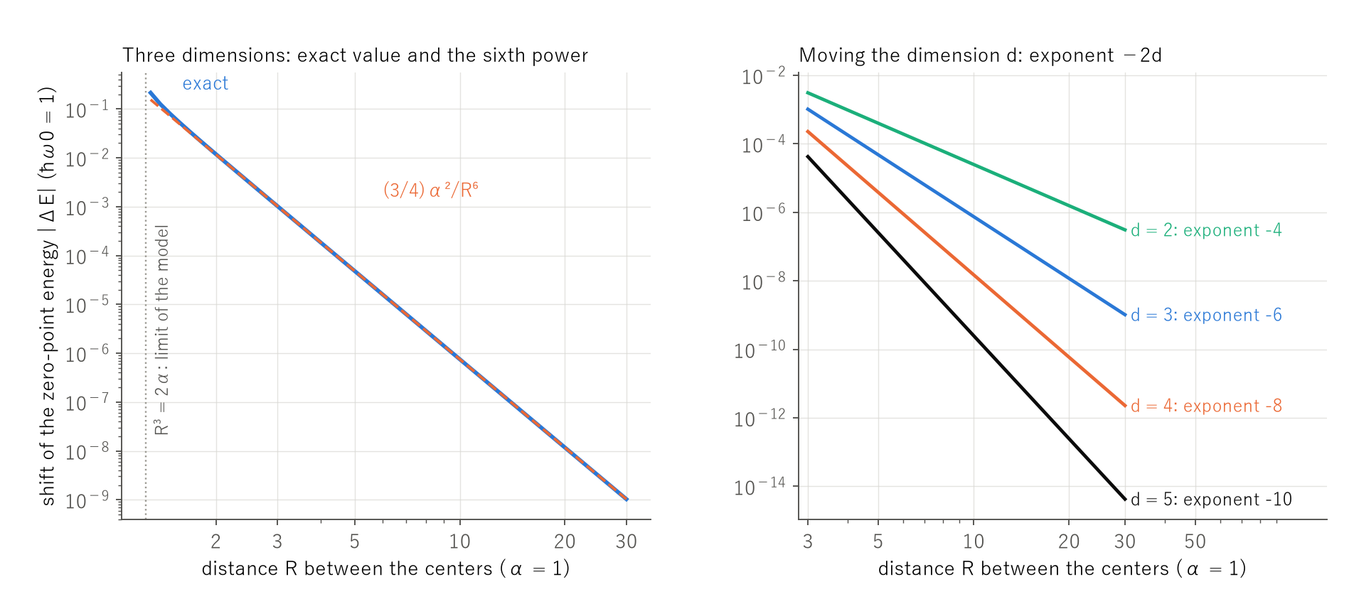
At $R=10$ the ratio is 1.000001, and the exponent from $R=10$ to 20 is $-6.000001$. The binding breaks down at $\kappa=1/2$ ($R^3=2\alpha$), and the model cannot treat closer distances. If the springs were classical, both would rest in the lowest-energy state, with no lopsidedness and no attraction. At zero temperature the attraction comes only from the zero-point motion.
The average lopsidedness stays $\langle z_A\rangle=0$ even with the coupling. The product, however, is not 0. At $\kappa=0.1$, $\langle z_Az_B\rangle=0.051291$, and sideways $\langle x_Ax_B\rangle=-0.025157$. Divided by the fluctuations with the coupling, $\langle z_A^2\rangle=0.507726$ and $\langle x_A^2\rangle=0.501889$, the correlation coefficients are 0.1010 along the joining line (same direction) and $-0.0501$ sideways (opposite directions); divided by the uncoupled 0.5 they would be 0.1026 and $-0.0503$. Since the zero-point state is Gaussian, the share of measurements that find the two lopsided the same way is $\frac12+\arcsin(\rho)/\pi$: 0.5322 for the same direction along the line, and 0.5160 for opposite directions sideways. Along the joining line the lopsidedness points the same way in both; sideways it points opposite ways. Both arrangements lower the energy between the dipoles. Averaging each from outside gives 0, but multiplying the two does not, and the attraction comes from there (Figure 1).
4. Retracing the Coefficient between Two Hydrogen Atoms
At large distances the attraction between two hydrogen atoms is $-C_6/R^6$. $C_6$ is set by the integral of the square of the polarizability at imaginary frequency,
$$C_6=\frac{3}{\pi}\int_0^\infty\alpha(i\omega)^2\,d\omega,\qquad \alpha(i\omega)=\sum_n\frac{f_n}{\Delta E_n^2+\omega^2} ,$$where $f_n$ is the oscillator strength from 1s to a p room and $\Delta E_n$ the energy difference. We solved the p rooms ($\ell=1$) in the basis $r^2e^{-r}L_k^{(4)}(2r)$ ($k=0,\dots,K-1$, with $L$ the Laguerre polynomials) and obtained a sequence of pseudo-states in which the bound levels and the continuum are made discrete together. This is a basis of the same form as the one Mitroy and Bromley (2005) used for the dispersion coefficients of hydrogen, and our calculation retraces theirs. The integrals are exact on Gauss–Laguerre points. In closed form, $C_6=\frac32\sum_{n,m}f_nf_m/(\Delta E_n\Delta E_m(\Delta E_n+\Delta E_m))$.
| basis size | lowest p level | sum of oscillator strengths | static polarizability | $C_6$ |
|---|---|---|---|---|
| 10 | $-0.1249999396$ | 1.0000000000 | 4.5000000000 | 6.4990267053 |
| 20 | $-0.1250000000$ | 1.0000000000 | 4.5000000000 | 6.4990267054 |
| 30 | $-0.1250000000$ | 1.0000000000 | 4.5000000000 | 6.4990267054 |
| 40 | $-0.1250000000$ | 1.0000000000 | 4.5000000000 | 6.4990267054 |
The sum of oscillator strengths 1 and the static polarizability 9/2 follow exactly from the construction of the basis, since 1s multiplied by $z$ and the first-order solution are in the basis from the start (with 1 basis function the sum is 1 and the polarizability 4.0; with 2, 4.5). What shows the convergence is the lowest p level and $C_6$. The lowest p level matches the formula’s $-1/8$ from 20 basis functions on. $C_6$ is 6.4990267053304 with 10 basis functions, the same to 13 digits as the 10-function column of the table of Mitroy and Bromley (6.4990267053305). From 20 on it is 6.4990267054, differing from the best value of the same table, 6.4990267054058, by $4.3\times10^{-14}$ with 20 basis functions and $1.7\times10^{-13}$ with 40. As another route, integrating the square of $\alpha(i\omega)$ numerically on 400 Gauss–Legendre points also gave 6.4990267054. $\alpha(i\omega)$ falls as 4.500000 at $\omega=0$, 1.905388 at 0.5, 0.742441 at 1 and 0.224474 at 2.
London’s simple formula keeps the polarizability at its true value $\alpha=9/2$ and puts only the excitation energy at a single value (the ionization energy $I=1/2$), writing $C_6\approx\frac34I\alpha^2$. For hydrogen this gives 7.593750, 1.168444 times the correct value. It comes out large because most of the true polarizability comes from transitions below $I$. The transition to 2p alone ($\Delta E=3/8$, $f=0.416197$) gives a polarizability of 2.959621, 0.657694 of 9/2. The energy of a single line that matches $C_6$ is $C_6/(\frac34\alpha^2)=0.427919$, below $I$, and the ratio 1.168444 is exactly $I\div0.427919$.
5. The Source of the Fluctuation: Zero Point or Heat
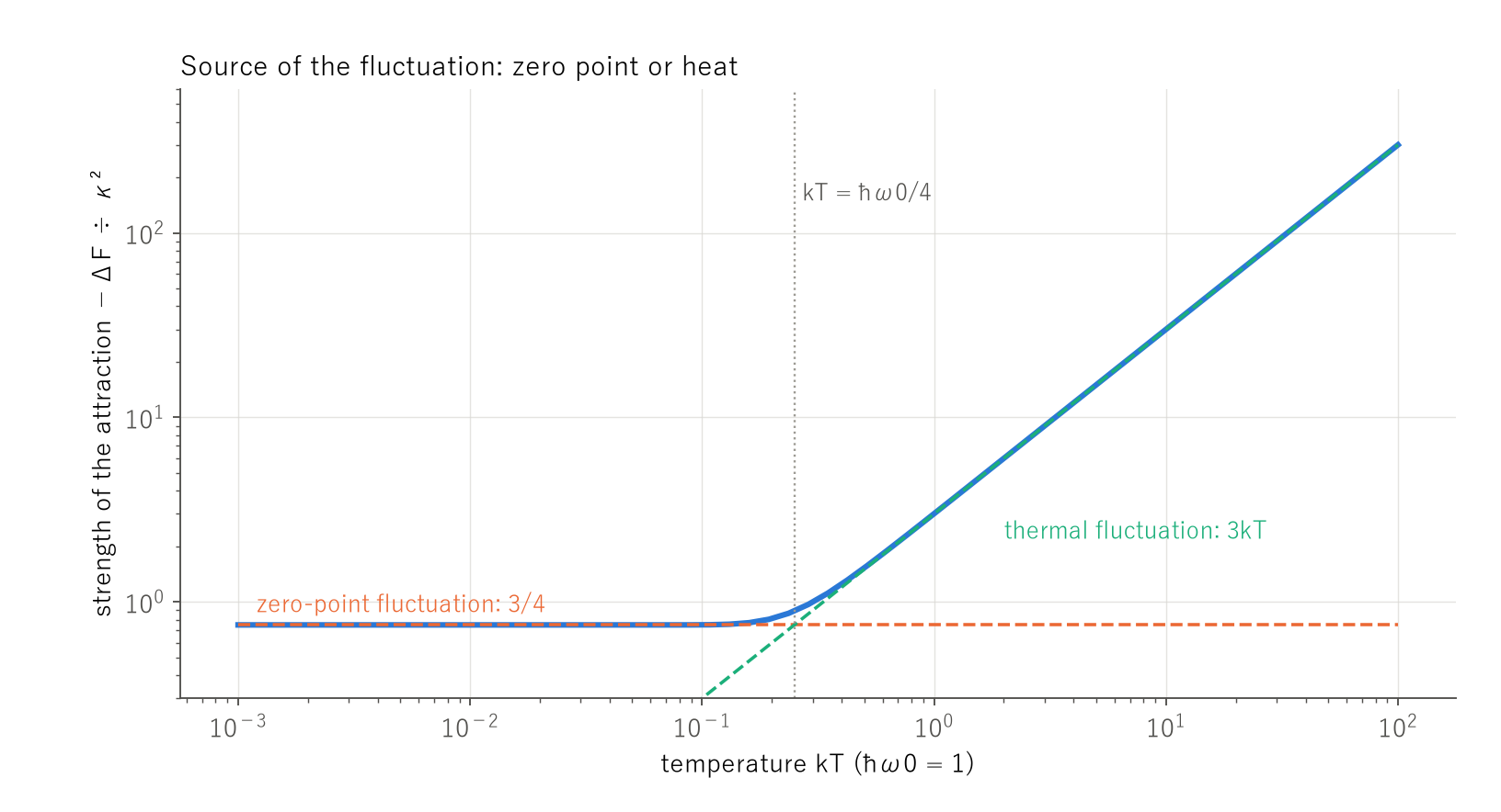
Placing the spring model at temperature $T$, the free energy is the sum over modes of $\frac12\omega+kT\ln(1-e^{-\omega/kT})$. With $\kappa=10^{-3}$ we divided the shift $\Delta F$ from the uncoupled value by $\kappa^2$.
| $kT$ ($\hbar\omega_0=1$) | $\Delta F/\kappa^2$ | thermal formula $-3kT$ |
|---|---|---|
| 0 | $-0.750001$ | 0 |
| 0.01 | $-0.750001$ | $-0.03$ |
| 0.1 | $-0.750750$ | $-0.3$ |
| 0.25 | $-0.892020$ | $-0.75$ |
| 1 | $-3.003980$ | $-3$ |
| 10 | $-30.000049$ | $-30$ |
| 100 | $-300.000450$ | $-300$ |
When $kT$ is far below $\hbar\omega_0$, $\Delta F/\kappa^2$ approaches $-3/4$ from the zero-point fluctuation; when far above, $-3kT$ from the thermal fluctuation. The thermal fluctuation also attracts in inverse proportion to the sixth power of the distance. What differs by source is the coefficient, and the two approximate formulas cross at $kT=\hbar\omega_0/4$ (Figure 2). There, however, the thermal addition is only $-0.142019$, 0.1592 of the whole $-0.892019$; the thermal addition equals the zero-point part $3/4$ at $kT=0.490228 \hbar\omega_0$. The thermal attraction comes not from the internal energy but from the entropy term: at $kT=1$, $\Delta U/\kappa^2=-0.015533$ and $\Delta F/\kappa^2=-3.003980$; at $kT=10$, $\Delta U/\kappa^2=-0.000017$ and $\Delta F/\kappa^2=-30.000049$. Taking the $\hbar\omega_0$ of an atom to be of the size of a hartree (27.211386 eV), room-temperature $kT=0.025852$ eV at 300 K is 0.000950 of it, so at distances short enough that delay does not matter, the zero-point fluctuation decides the attraction of atomic electron clouds.
6. Moving the Dimension
In $d$ dimensions the potential of a charge weakens as $1/R^{d-2}$ (logarithmically for $d=2$), that of a dipole as $1/R^{d-1}$, and the field of a dipole as $1/R^d$. Writing the coupling between dipoles as $\kappa(\delta_{ij}-d n_in_j)$ with $\kappa=\alpha/R^d$, the eigenvalues of the coupling are 1 sideways ($d-1$ of them) and $1-d$ along the joining line, and the squared frequencies are $1\pm\kappa$ ($d-1$ pairs) and $1\pm(d-1)\kappa$ (one pair). For small $\kappa$ the shift is $-d(d-1)\kappa^2/8$. The normalization of the coupling is a choice of the model; what we check here are the exponent and the ratio.
| dimension $d$ | $\Delta E\div(-d(d-1)\kappa^2/8)$ | exponent for $R=10\to20$ | formula $-2d$ |
|---|---|---|---|
| 2 | 1.000000 | $-4.000042$ | $-4$ |
| 3 | 1.000000 | $-6.000001$ | $-6$ |
| 4 | 1.000000 | $-8.000000$ | $-8$ |
| 5 | 1.000000 | $-10.000000$ | $-10$ |
Since $\kappa$ goes as $R^{-d}$, the shift goes as $R^{-2d}$. The 6 of three dimensions is the exponent 3 of the dipole field, doubled by the square. Paper 1106 showed that a physical infinity is set by a contest between the exponent of thinning and the dimension. Here too the exponent comes from the dimension, but the exponent of the attraction is twice the dimension, doubled by the square.
7. Why Is the van der Waals Force Weak?
Paper 278 cut the classes of chemical bond by strength and temperature and showed that only the van der Waals force falls below $RT$ at room temperature. Its scope note said that it does not treat at all why it is weak. What this paper answers is the weakness of the dispersion part of the van der Waals force (it does not enter the forces between permanent dipoles). In the numbers of this paper, the weakness has two steps. The average lopsidedness of one atom is 0, so there is no first-order attraction. What remains is the second order, the product of two fluctuations, which acts through the square of the small ratio $\kappa=\alpha/R^3$. Even real hydrogen ($\alpha=4.5$) at 6 Bohr radii has $\kappa=0.0208$, and at 8 Bohr radii 0.0088. Even with $\kappa=0.1$ in the spring model, the shift is only 0.007572 of $\hbar\omega_0$, 0.005048 of the zero-point energy 1.5 of one oscillator.
The scattering cross section of Rayleigh scattering in Paper 1089 also contains the square of the polarizability. There it is the light sent out by the induced lopsidedness of one particle; here it is the product of the fluctuations of two atoms. The polarizability $\alpha$ is also the quantity used with the local field in Paper 1097, and the same $\alpha$ enters both the blue of the sky and the attraction of noble gases. As in the judgement of Paper 300, the same $\alpha^2$ appearing in two formulas does not by itself make them share a root.
8. The Separator
The separator is whether the numbers read from outside are taken as the average of one atom or as the product of the fluctuations of two atoms. Taken as averages, all the numbers of a round atom are 0 and there is no attraction; these are the first-order numbers counted in Paper 1107. Taken as products, they are not 0, and the attraction remains as $\kappa^2$, in inverse proportion to the sixth power of the distance. A second dividing line is the source of the fluctuation: zero point or heat splits the coefficient into $\frac34\hbar\omega_0$ and $3kT$, and the two approximate formulas cross at $kT=\hbar\omega_0/4$. The thermal attraction comes from the entropy term.
Closing
An atom with a full shell is round on average and sends nothing out. Yet atoms attract each other. What attracts is not the average shape: the fluctuation of the electron, which a measurement finds lopsided toward somewhere, lines up between the two atoms, and the strength goes as the square of the small ratio α/R³, in inverse proportion to the sixth power of the distance. Retracing the coefficient between two hydrogen atoms in a basis of the same form as Mitroy and Bromley gives 6.4990267054, and London’s simple formula comes out 1.168444 times larger because most of the polarizability comes from 2p, below the ionization energy. In atoms the source of the fluctuation is the zero point, and the thermal addition equals the zero-point part only at kT = 0.490228ħω0. The 6 is twice the exponent 3 of the dipole field, and becomes 2d in d dimensions. The dispersion force is weak because the first order is 0 and only the second order remains.
References
- Casimir, H. B. G., and Polder, D. (1948). The influence of retardation on the London-van der Waals forces. Physical Review.
- London, F. (1930). Zur Theorie und Systematik der Molekularkräfte. Zeitschrift für Physik.
- Mitroy, J., and Bromley, M. W. J. (2005). The higher-order $C_n$ dispersion coefficients for hydrogen. Physical Review A.
- Yamagishi, Y. (2026). The Classes of Chemical Bond Are a Continuum of Strength Cut by a Temperature [Paper 278]. YOI: https://www.yamagishiyuuki.com/yoi/278; DOI: 10.5281/zenodo.22170205
- Yamagishi, Y. (2026). The Three Hundredth Census: Whether Two Things Share a Root Is Decidable [Paper 300]. YOI: https://www.yamagishiyuuki.com/yoi/300; DOI: 10.5281/zenodo.22171914
- Yamagishi, Y. (2026). “Colloid” Is Not the Name of a Substance but of a Window in Size [Paper 673]. YOI: https://www.yamagishiyuuki.com/yoi/673; DOI: 10.5281/zenodo.23014755
- Yamagishi, Y. (2026). The 32, 64 and 128 That Stand Next to π Are Small Numbers from Integrals Times Powers of Two from Diameter and Wavelength [Paper 1089]. YOI: https://www.yamagishiyuuki.com/yoi/1089
- Yamagishi, Y. (2026). A Lattice Sum of Dipole Fields Is Decided by the Shape of the Summation: 0 for a Sphere, 4π/3 for a Thin Needle, −8π/3 for a Thin Plate [Paper 1097]. YOI: https://www.yamagishiyuuki.com/yoi/1097
- Yamagishi, Y. (2026). A Physical Infinity Is Set by How Fast Things Thin Out against the Dimension, Not by the Mass [Paper 1106]. YOI: https://www.yamagishiyuuki.com/yoi/1106
- Yamagishi, Y. (2026). When the Field Equation Is of Second Order, the Interior Can Be Read from Outside a Closed Skin Only as One Number per Angular Pattern [Paper 1107]. YOI: https://www.yamagishiyuuki.com/yoi/1107
Reference
Yamagishi, Y. (2026). Atoms That Are Round on Average Still Attract, Their Fluctuating Lopsidedness Lining Up, in Inverse Proportion to the Sixth Power of the Distance [Paper 1109]. YOI: https://www.yamagishiyuuki.com/yoi/1109
ORCID: 0009-0006-8587-3450
PDF (English) · PDF (Japanese) · Date proof of the English PDF (OpenTimestamps .ots) · SHA256SUMS
The record page for this paper (in Japanese, with the PDFs in each language and the date proof): YOI 1109. This paper is a preprint and has not been peer reviewed.