[Paper 1111] The Inverse Square Hides the Interior from a Static Field and Carries the Echo of a Wave Undistorted

Abstract

Paper 1107 counted that, for a field obeying a local equation of second order, the interior can be read from outside a closed skin only as one number per angular pattern. The inverse-square field of gravity or electricity is the representative case: there is no source outside the interior, and the flux through any closed surface, whatever its shape, is 4π times the amount inside. This 4π comes from the field being massless, and its root differs from that of one number per pattern (Paper 1107). This paper extends the same count to frequency bands and to measurements with a sending point added, and puts on one table the scattering-field theory of Kenjiro Kimura and colleagues at Kobe University (measure while moving both the point that sends and the point that receives, and image the interior by solving the equation that the function of the two points obeys) and the inverse square of the uniqueness theorem (Paper 01).

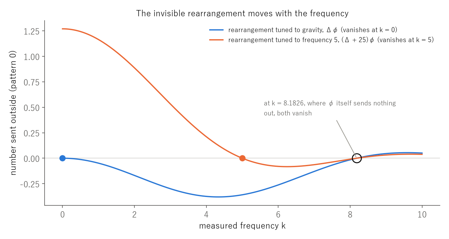
When we measure by receiving only, with no point that sends, what goes outside is one number per pattern, for a static field and for one frequency alike (that it is one at a single frequency was also counted for the Helmholtz kernel in Paper 1107). Building the field at 30 outside radii by numerically integrating the kernel, the second singular value was at most 2.24×10⁻¹⁴ of the largest in all 16 cases. What reaches far away at one frequency is the value of the Fourier transform of the interior on the sphere of radius k. The invisible rearrangement has the form (Δ + k0²)φ: at frequency k0 it sends nothing out, and at other frequencies it does, weighted by (k0² − k²). The Δφ of Paper 1107 is k0 = 0, and the rearrangement of the Yukawa field corresponds to an imaginary k0. At a frequency where φ itself sends nothing out (8.182561 for φ = (1 − r²)³), every (Δ + k0²)φ built from the same φ is invisible. If one measures only at finitely many frequencies, a rearrangement of the multiplied form stays invisible at all of them, but once the frequency is moved over an interval, the only invisible rearrangement is zero.

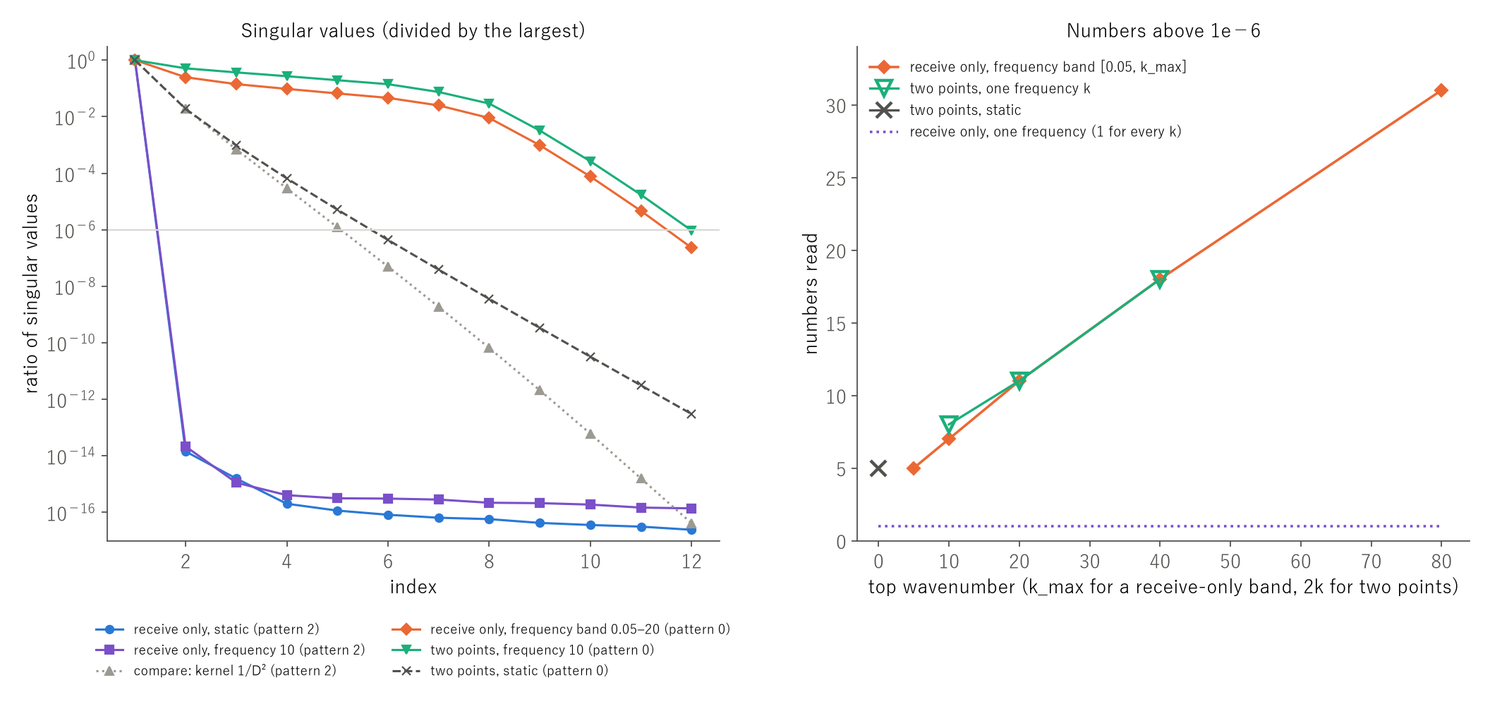
Receiving only and moving the frequency over a band, the number that can be read grows by about one each time the top of the band grows by π, and thins out gradually rather than at a cliff (for pattern 0, the numbers above 10⁻⁶ of the largest are 5, 7, 11, 18 and 31 for tops 5, 10, 20, 40 and 80). Adding a sending point does the same. Moving the point that sends and the point that receives on a skin of radius 1.5, with a spherically symmetric interior that bounces the wave once, one frequency k = 5, 10 and 20 reads 8, 11 and 18 numbers, nearly the 7, 11 and 18 read by receiving only over the band [0, 2k]. The reason is that in the far field the quantity measured with two points becomes exactly the quantity measured by receiving only over the band [0, 2k]. Two static points read 5 numbers, but their singular values fall fast.

Kimura and colleagues derived the equation that the scattering field obeys as a function of two points (equation (2-5) of the Kokyuroku paper) as an approximation for short wavelengths. In our check, this (2-5), in which the points that send and receive share only the coordinate x, holds without approximation for the single-scattering kernel. The operator is the formula that eliminates the split transverse wavenumbers from the dispersion relations of the outgoing and returning waves; like the double-square-root equation of seismic exploration, it rests on each leg travelling freely. At 40 digits the remainder is below 10⁻⁴¹ of the size of the terms, while for a product with a shifted frequency or a product of static kernels it is 0.148 to 1.000. The approximation works at the step that brings the depths of the sending and receiving points together to fit one measured surface (equations (2-13) and (2-14)), where the stationary-phase point, at which the wavenumbers of the two legs are parallel, is chosen. Since the strength of the scatterers does not enter the equation, it can be solved inwards from the measured values alone. The image stands only where the points that send and receive meet a scatterer and the time returns to zero, that is, where the premise of the equation, an empty region, no longer holds; in the limit where all frequencies are present it is sharp at one point.

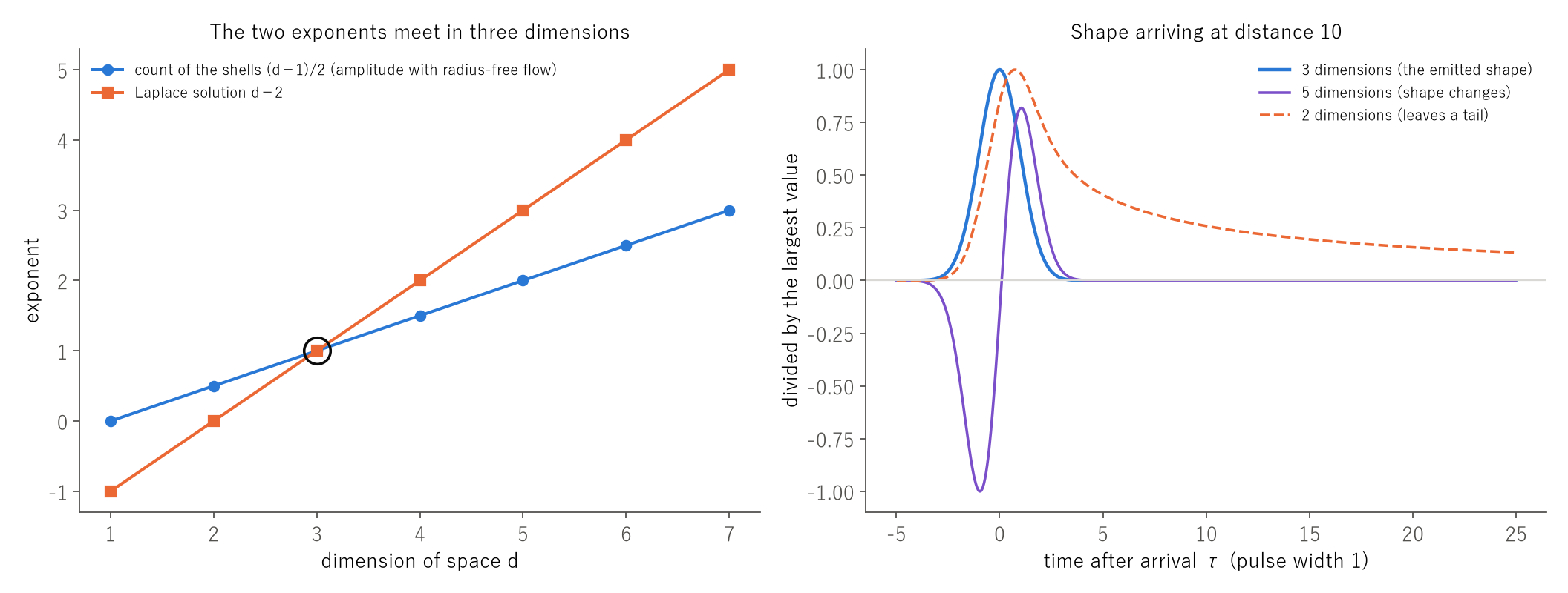
On the side of the echo, the inverse square plays another role. That the flow of an outgoing spherical wave does not depend on the radius fixes the amplitude at 1/r, and when the point that sends and the point that receives are separated, the strength of one bounce is divided by (4π)² and the product of the two distances, and the arrival time is the sum of the paths. Even on a spheroid of equal arrival time the strength changes: at the vertex and the co-vertex of its cross-sectional ellipse with path sum 4 and foci 2 apart, the squared strengths differ by a factor of 1.777778. For a spherical wave whose amplitude falls as the (d − 1)/2 power of the distance to arrive undistorted in d dimensions, the remainder is (d − 1)(3 − d)/4, which vanishes in one and three dimensions. One dimension is a plane wave whose amplitude does not weaken; a wave that weakens with distance while keeping its shape exists only in three dimensions, where the flux-keeping exponent (d − 1)/2 and the Laplace exponent d − 2 meet. In five dimensions the correlation between the arriving shape and the emitted shape at distance 10 is 0.688416, approaching 0.606531 far away.

The separator is whether what is measured outside fits into one function on the skin. If it fits, what goes outside is one number per pattern and stops as at a cliff; once a frequency band or a sending point carries the measurement beyond the dimension of the skin, the numbers grow gradually and reach the interior. The inverse-square field is the representative of fields that hide the interior from outside when static, and for a wave it carries the echo there and back undistorted, only in three dimensions. The method of Kimura and colleagues can read the interior because what it measures with two points exceeds the dimension of the skin; that three dimensions keep the shape makes the reading of arrival times as paths straightforward.

Keywords: inverse source problem, inverse scattering problem, nonradiating source, multi-frequency data, diffraction tomography, Huygens principle, spherical wave, separator.

Scope (what is not claimed)

This paper claims no new theorem and no new law. That sources exist which send nothing out at one frequency, so that the inverse source problem is not unique, is in Devaney and Wolf (1973) and Bleistein and Cohen (1977); that moving the frequency determines the source uniquely, with stability that increases as the band widens, is in Bao, Lin and Triki (2010); that a field at one frequency has effectively finitely many degrees of freedom is in Bucci and Franceschetti (1989); that moving the incident and receiving directions (plane waves, far field) reads the interior up to the sphere of radius 2k (diffraction tomography) is in Wolf (1969); and that the far field is the Fourier transform of the interior on a sphere is standard. That, when receiving only, the count stops at one per pattern for the Helmholtz kernel too, and that the rearrangement tuned to the Yukawa field is invisible, were counted in Paper 1107. That two static points (a boundary map) determine the interior is the problem of Calderón (1980) and of Sylvester and Uhlmann (1987), treated in Paper 99. Huygens’ principle in odd dimensions of three or more is in Paper 247, Paper 64 and Courant and Hilbert (1962), the round-trip 1/r⁴ in Paper 335, the range resolution c/2B in Paper 802, and that conservation of the flow of a spherical wave fixes the exponent 2 in Paper 41 and Paper 53. That a spherical wave weakening with distance while keeping its shape exists only in three dimensions is a classical computation, also found among the exercises of textbooks on partial differential equations. Forming images on the premise that the wave equation holds in the coordinates of the sending point and of the receiving point separately, and the double-square-root equation that adds the vertical wavenumbers of the two legs, are known in seismic exploration (Yilmaz and Claerbout 1980; Claerbout 1985), and placing the image where downgoing and upgoing waves meet in time and place is in Claerbout (1971). The scattering-field theory is that of Kimura and Kimura (2021); we read RIMS Kokyuroku 2186, the arXiv paper of Yabumoto, Yumii and Kimura (2025) and the European patent application of Kimura and colleagues (2024), and not their other papers. We have not checked whether Kimura and colleagues wrote elsewhere that equation (2-5) holds exactly for the single-scattering kernel. We look only at scalar waves, corresponding to one component of sound or light, and do not treat polarization, multiple scattering, dispersion and attenuation in the medium, models of noise and estimates of stability, the computation and devices that form images, medical performance, or the magnetic imaging of batteries. The numbers that can be read are counts of singular values above thresholds, and they move when the threshold moves. What we add is the following: we extended the pattern-by-pattern count of Paper 1107 to frequency bands and to a sending point, and counted on one table that, receiving only, the count stops at one per pattern as at a cliff, while a band or two points make it grow gradually; we checked, with a far-field identity, that for a spherically symmetric interior two points at one frequency k read about as many numbers as receiving only over the band [0, 2k]; we lined up the rearrangement of Paper 1107 and that of the Yukawa field as members of a family of invisible rearrangements that moves with the frequency, and counted that with finitely many frequencies a multiplied form remains; we checked that the equation (2-5) of Kimura and colleagues is the formula that eliminates the split transverse wavenumbers from two dispersion relations, that it holds without approximation for the single-scattering kernel, and that the approximation enters as stationary phase at the step (2-13), (2-14) that brings the depths together; we counted the strength and the time of an echo with separated points of sending and receiving; and we placed the spherical wave that weakens while keeping its shape in three dimensions, as the meeting of the flux-keeping exponent and the Laplace exponent. Paper 89, in its scope (what it does not show), made no new prediction and quarantined the kinship of the angling technique, the Universe OS and Professor Kimura’s inverse problem as a Layer-3 personal note. This paper takes that seat and moves to Layer 2 the part of the kinship that can be said in numbers: that the equation of Kimura and colleagues describes only how waves travel through an empty region, and that the image stands only where the premise of that equation, an empty region, no longer holds. We do not treat the angling technique. The scope note of Paper 335 said that it does not enter arrangements with sending and receiving separated (bistatic). This paper takes that seat and counts the strength and the time of an echo with the point that sends and the point that receives separated.

1. Can the Outside Read Only One Skin’s Worth of Numbers?

Paper 1107 counted that, if a field obeys a local equation of second order, the interior can be read from outside a closed skin only as one number per angular pattern. The finer the interior is cut, the more of it is invisible from outside. Yet there are techniques that image the interior from outside. Kenjiro Kimura and colleagues at Kobe University measure while moving both the point that sends a wave and the point that receives it, and image the interior by solving, with the values on the measured surface as boundary conditions, the equation that the scattering field obeys as a function of the two points (Kimura and Kimura 2021; Yabumoto, Yumii and Kimura 2025). Paper 89 quarantined the kinship with this inverse problem as a Layer-3 personal note. This paper places the part of it that can be said in numbers on the count of Paper 1107.

We name two ways of measuring. Measuring the field that the interior sends out, anywhere outside, with no point that sends, we call measuring by receiving only; there may be any number of receiving points. Moving two points, one that sends a wave and one that receives it, and measuring the wave that the interior has bounced once, we call measuring with two points. The receive-only question reads the sources inside and the two-point question reads the strength of the bounce; they are different questions, and what this paper lines up is how many numbers each can read from outside.

Let the interior lie inside a ball of radius 1, and split it by angular pattern (spherical harmonic $Y_{\ell m}$) into functions of the radius $\rho_{\ell m}(r)$. The field measured outside obeys $\Delta u=-\rho$ if it is static, and $(\Delta+k^2)u=-\rho$ for each wavenumber $k$ (called the frequency below) if it is a wave. The kernels are $1/(4\pi D)$ and $e^{ikD}/(4\pi D)$, with $D$ the distance between two points.

2. Receiving Only: One per Pattern, Static or at One Frequency

Expanding the kernel, the field at a point $\mathbf x$ outside the skin ($|\mathbf x|>1$) is

$$u(\mathbf x)=\sum_{\ell,m}c_{\ell m}\,h_\ell(k|\mathbf x|)\,Y_{\ell m}(\hat{\mathbf x}),\qquad c_{\ell m}=ik\int_0^1\rho_{\ell m}(r)\,j_\ell(kr)\,r^2\,dr$$

($j_\ell$ and $h_\ell$ are the spherical Bessel function and the spherical Hankel function of the first kind). For a static field, $h_\ell(k|\mathbf x|)$ becomes $|\mathbf x|^{-\ell-1}$ and $ik j_\ell(kr)$ becomes $r^\ell/(2\ell+1)$. However many outside points are taken, what goes out from the pattern $(\ell,m)$ is the one number $c_{\ell m}$, and the dependence on the outside radius is only the fixed shape of $h_\ell$. Paper 1107 counted that the count stops at one per pattern for the Helmholtz kernel too. This paper rechecks it along the outside radius and, from the next section on, moves to frequency bands and a sending point.

We divided the interior into 40 layers along the radius and built the field at 30 outside radii on the z axis (1.2 to 3.0) by numerically integrating the kernel over the angles, without using the expansion. Listing the singular values of the table of 30 rows and 40 columns, in each of the 16 cases (static and frequencies 2, 5 and 10, patterns 0 to 3) the second singular value was at most $2.24\times10^{-14}$ of the largest, and one number went out. The numerical integration agreed with the expansion to within $2.1\times10^{-13}$. For comparison, with the kernel $1/(4\pi D^2)$ (on the side of power kernels whose count does not stop, in Paper 1107), singular values above $10^{-10}$ of the largest continue to 8 for pattern 0 and 7 for pattern 2 (Figure 1, left).

The amplitude that reaches far away at one frequency is the Fourier transform of the interior, read on the sphere of radius $k$.

$$\lim_{R\to\infty}R\,e^{-ikR}\,u(R\hat{\mathbf x})=\frac{1}{4\pi}\,\hat\rho(k\hat{\mathbf x}),\qquad \hat\rho(\mathbf q)=\int\rho(\mathbf y)\,e^{-i\mathbf q\cdot\mathbf y}\,d\mathbf y$$

For a blob of width 0.1 placed off centre at $(0.3, 0.1, -0.2)$, with the field integrated at $R=1000$ and 2000, the difference from the right side was at most $3.698\times10^{-4}$ and $1.849\times10^{-4}$; doubling $R$ divides it by 2.0002. What one frequency reads is one skin of radius $k$ in Fourier space. The multipoles of a static field correspond to reading one coefficient per pattern from the expansion of the Fourier transform about the origin.

3. The Invisible Rearrangement Moves with the Frequency

Paper 1107 checked that rearranging the interior of a cube in the form $\Delta\varphi$ does not change the gravity outside ($\varphi$ is a smooth hill that lives only inside). Waves have the same form.

$$\rho=(\Delta+k_0^2)\,\varphi$$

A rearrangement of this form sends nothing out at frequency $k_0$, because the solution of the wave equation is $u=-\varphi$, which is zero outside the skin. At another frequency $k$, integration by parts gives what goes out as

$$\int(\Delta+k_0^2)\varphi\;j_\ell(kr)\,Y^{*}_{\ell m}\,d\mathbf y=(k_0^2-k^2)\int\varphi\;j_\ell(kr)\,Y^{*}_{\ell m}\,d\mathbf y .$$

The $\Delta\varphi$ of Paper 1107 is the case $k_0=0$, and the $(\Delta-\kappa^2)\varphi$ of the Yukawa field is the case of an imaginary $k_0=i\kappa$. With $\varphi=(1-r^2)^3$ (pattern 0), we list what goes out, $\int\rho j_0(kr) r^2 dr$ ($\int\rho r^2 dr$ at $k=0$).

rearrangement	$k=0$	$k=2$	$k=5$	$k=8$
$\Delta\varphi$	$-0.0000000$	$-0.1689527$	$-0.3590739$	$-0.0156601$
$(\Delta+25)\varphi$	$1.2698413$	$0.8870017$	$-0.0000000$	$-0.0095429$

Every value agreed with the identity of integration by parts. For pattern 2 ($\varphi=r^2(1-r^2)^3$), too, $(\Delta+25)\varphi$ vanished only at $k=5$ among the four frequencies of the table. The rearrangements tuned to the Yukawa field, with $\kappa=1$ as in Paper 1107 (and 3), sent out less than $10^{-16}$ into the Yukawa field, while $\Delta\varphi$ of the same $\varphi$ (the rearrangement tuned to gravity) did send out into the Yukawa field. The equation that governs the outside field decides the form of the invisible rearrangement.

The invisible frequency need not be single. At a frequency where $\varphi$ itself sends nothing out ($\int\varphi j_0(kr) r^2 dr=0$, $k=8.182561$ for this $\varphi$), no $(\Delta+k_0^2)\varphi$ built from the same $\varphi$ goes out (Figure 2). If one measures only at finitely many frequencies $k_1,\dots,k_n$, a rearrangement of the form $(\Delta+k_1^2)\cdots(\Delta+k_n^2)\psi$ stays invisible at every one of them. Building $(\Delta+9)(\Delta+36)\psi$ with $\psi=(1-r^2)^5$, what goes out is $7.3\times10^{-16}$ at $k=3$ and $-7.9\times10^{-16}$ at $k=6$, but $-2.4885531$ at $k=4.5$ in between. If the frequency is moved over an interval, the only invisible rearrangement is zero. What goes out is the value of the Fourier transform of the interior on a sphere, and moving over an interval fixes those values on a whole spherical shell. When the interior lies only inside a ball, its Fourier transform is everywhere a power series (it is analytic), so if it vanishes on a shell it vanishes everywhere. The form of sources that send nothing out at one frequency is treated by Devaney and Wolf (1973) and Bleistein and Cohen (1977), and uniqueness when the frequency is moved, with stability that increases as the band widens, by Bao, Lin and Triki (2010).

4. Moving the Frequency: The Numbers Grow Gradually

Still receiving only, we move the frequency over 400 values of the band $[0.05, k_{\max}]$, so that the number that goes out of each pattern is lined up as many times as there are frequencies. Dividing the interior into 60 layers along the radius, we built the table and counted the singular values above $10^{-3}$, $10^{-6}$ and $10^{-9}$ of the largest.

$k_{\max}$	$k_{\max}/\pi$	pattern 0 ($10^{-3}$, $10^{-6}$, $10^{-9}$)	pattern 2 ($10^{-3}$, $10^{-6}$, $10^{-9}$)
5	1.59	4, 5, 7	3, 5, 6
10	3.18	5, 7, 9	5, 7, 8
20	6.37	8, 11, 13	8, 10, 12
40	12.73	15, 18, 20	14, 17, 20
80	25.46	27, 31, 33	27, 30, 33

The number that can be read grows by about one each time the top of the band $k_{\max}$ grows by $\pi$; $k_{\max}/\pi$ is the number of half wavelengths that fit in the radius 1. Where to cut depends on the size of the noise (the threshold), and the singular values thin out gradually rather than at a cliff. For pattern 0 over the band $[0.05, 20]$, the ratio of neighbouring singular values down to $10^{-9}$ of the largest is at least 0.041, a different order altogether from the cliff of receiving only at one frequency (at most $2.24\times10^{-14}$; Figure 1). That a field at one frequency has effectively finitely many degrees of freedom was shown by Bucci and Franceschetti (1989), and that moving the frequency determines the source, with stability that increases as the band widens, by Bao, Lin and Triki (2010). This paper lines up the cliff and the gradual fall on the same measure as Paper 1107.

5. Adding a Second Point

Next, we move two points, the point that sends and the point that receives, on a skin of radius 1.5. The interior bounces the wave only once (the Born approximation), and the strength of the bounce is put in a spherically symmetric (pattern 0) $\varepsilon(r)$. The signal that leaves the sending point $\mathbf s_1$ and reaches the receiving point $\mathbf s_2$ is

$$u(\mathbf s_1,\mathbf s_2)=\int\varepsilon(\mathbf y)\,G(\mathbf s_1,\mathbf y)\,G(\mathbf y,\mathbf s_2)\,d\mathbf y$$

($G$ is the kernel of the previous section, and factors such as $k^2$ are included in $\varepsilon$). Expanding the kernel and integrating over a shell gives a function of the angle $\gamma$ between the two points alone,

$$u=\sum_{\ell}\frac{2\ell+1}{4\pi}\,P_\ell(\cos\gamma)\int_0^1\varepsilon(r)\,g_\ell(r)^2\,r^2\,dr,\qquad g_\ell(r)=ik\,j_\ell(kr)\,h_\ell(1.5k)$$

($g_\ell=r^\ell/((2\ell+1) 1.5^{\ell+1})$ for a static field). From the pattern-0 interior, one number per $\ell$, weighted by $j_\ell(kr)^2$, goes out. The numerical integration over the shell and this sum ($\ell\le120$) agreed to within $5.3\times10^{-14}$. Dividing the interior into 60 layers, we built the table at 160 points of $\cos\gamma$ and counted.

measurement (pattern-0 interior, 60 layers)	$10^{-3}$	$10^{-6}$	$10^{-9}$
receive only, one frequency (any $k$)	1	1	1
two points, static	2	5	8
two points, frequency $k=5$	6	8	10
two points, frequency $k=10$	9	11	14
two points, frequency $k=20$	16	18	21

Receiving only at one frequency reads a single number for pattern 0, but two points read many layers even at one frequency. At the line $10^{-6}$, the 8, 11 and 18 for $k=5$, 10 and 20 are nearly the 7, 11 and 18 read by receiving only over the band $[0.05, 2k]$ (Figure 1, right). The reason shows in the far field. Far away, $h_\ell(kR)^2$ approaches $(-1)^\ell h_0(kR)^2$ (multiplying $kR$ by 10 divides the difference by 10.0000), and since

$$\sum_{\ell}(2\ell+1)(-1)^\ell j_\ell(kr)^2P_\ell(\cos\gamma)=j_0\bigl(2kr\cos(\gamma/2)\bigr)$$

(difference at most $1.2\times10^{-15}$), the pattern-0 quantity measured with two points becomes exactly the quantity measured by receiving only at the wavenumber $2k\cos(\gamma/2)$. As $\gamma$ moves from 0 to $\pi$, that wavenumber moves from $2k$ to 0. This is the pattern-0 case of diffraction tomography (Wolf 1969), which reads the interior up to the sphere of radius $2k$ by moving the incident and receiving directions (plane waves, far field). A skin of radius 1.5 is not in the far field, so near-field parts are added. That is why two static points still read 5 numbers; this belongs with the Calderón problem, reading the interior from a boundary map (Paper 99). The interior is determined, but the singular values fall fast (the dashed line in Figure 1, left), and the reading is weak against noise.

6. The Scattering-Field Equation of Kimura and Kimura

Kimura and Kimura (2021) wrote the scattering field as a function of two points, the point $\mathbf r_1$ that sends and the point $\mathbf r_2$ that receives:

$$G(\mathbf r_1,\mathbf r_2,\omega)=\iiint\frac{e^{ikD_1}}{D_1}\,\frac{e^{ikD_2}}{D_2}\,\varepsilon(\xi)\,d\xi$$

($D_1$ and $D_2$ are the distances from the scattering point $\xi$ to the points that send and receive, written $\rho_1$ and $\rho_2$ in the Kokyuroku paper). The two points share only the $x$ coordinate, $\mathbf r_1=(x,y_1,z_1)$ and $\mathbf r_2=(x,y_2,z_2)$. They derived, by an approximation that drops the higher terms in $1/\rho$, that this function satisfies

$$\Bigl[\frac{1}{4}\Delta_5^{\,2}-(ik)^2\,\partial_x^2-(\partial_{y_1}^2+\partial_{z_1}^2)(\partial_{y_2}^2+\partial_{z_2}^2)\Bigr]G=0$$

($\Delta_5$ is the Laplacian in the five directions $x$, $y_1$, $z_1$, $y_2$ and $z_2$; equation (2-5) of the Kokyuroku paper, where $G$ is written $\phi$). With the values on the measured surface as boundary conditions they solved it inwards in the space of two points, brought the two points to the same point by $y_1\to y_2$ and $z_1=z_2$, and summed over frequencies (returning the time to zero) to obtain the image (equation (3-12)).

In our check, this (2-5) holds without approximation for the single-scattering kernel. The reason is short. Split $x$ into two, and regard the outgoing factor $A=e^{ikD_1}/D_1$ as a function of $(x_1,y_1,z_1)$ and the returning factor $B=e^{ikD_2}/D_2$ as a function of $(x_2,y_2,z_2)$. The factor $A$ satisfies $(\partial_{x_1}^2+\partial_{y_1}^2+\partial_{z_1}^2+k^2)A=0$, $B$ satisfies an equation of the same form, and setting $x_1=x_2=x$ at the end turns $\partial_x$ into $\partial_{x_1}+\partial_{x_2}$. Replacing $\partial_{y_1}^2+\partial_{z_1}^2$ in the operator by $-(k^2+\partial_{x_1}^2)$ and $\partial_{y_2}^2+\partial_{z_2}^2$ by $-(k^2+\partial_{x_2}^2)$ gives

$$\bigl(\partial_{x_1}\partial_{x_2}-k^2\bigr)^2+k^2\bigl(\partial_{x_1}+\partial_{x_2}\bigr)^2-\bigl(k^2+\partial_{x_1}^2\bigr)\bigl(k^2+\partial_{x_2}^2\bigr)=0,$$

which vanishes identically. The operator is the formula that eliminates the split transverse wavenumbers from the two dispersion relations of the outgoing and returning waves, and it uses nothing but that each leg travels freely. The idea of forming images on the premise that the wave equation holds in the coordinates of the sending point and of the receiving point separately is the same as in the double-square-root equation of seismic exploration, which sinks the sending and receiving points together (Yilmaz and Claerbout 1980; Claerbout 1985). Except at points with $D_1=0$ or $D_2=0$, the kernel satisfies (2-5) exactly. Computed at 40 digits at two points and two frequencies (3 and 7.5), the remainder of the equation was below $10^{-41}$ of the size of the terms. For comparison, a product with the frequency of the return alone multiplied by 1.3 gives 0.148 and 0.181, and applying the operator of frequency 3 to the product of static kernels $1/(D_1D_2)$ gives 1.000 and 0.272, not zero.

The approximation actually works at the step that brings the depths of the sending and receiving points together to fit one measured surface. The $s_1$ and $s_2$ of equation (2-14), used for $z_1=z_2$, are the vertical wavenumbers of two plane waves that split the transverse wavenumber $k_x$ between the outgoing and returning legs in the ratio $a:b$ ($a=\sqrt{k^2-k_{y_1}^2}$, $b=\sqrt{k^2-k_{y_2}^2}$); over 2000 cases the departure from the dispersion relations was at most $4.4\times10^{-16}$, and the remainder of equation (2-12) was $5.0\times10^{-15}$. This split is the one that makes $s_1+s_2$ largest for a given $k_x$, the stationary-phase point at which the $(x,z)$ wavenumbers of the two legs are parallel, and the $s_1+s_2$ of equation (2-13) is that maximum (over 400 cases the difference from the maximum was $1.9\times10^{-11}$ and the departure from parallel $1.1\times10^{-15}$). The European patent application for the same theory (Kimura, Kimura and Kimura 2024) writes, for an arrangement on a flat boundary in which the sending and receiving points share both $x$ and the depth $z$ (section II-1), that the kernel “may be regarded as almost an exact solution” of the equation there. When two coordinates are shared, the sum of the wavenumbers of the two legs fills an annulus in the plane, so in that arrangement no exact equation with constant coefficients seems to exist, and “almost” appears to be just right (our view). What this paper checked is (2-5), in which only $x$ is shared.

This equation does not contain the strength $\varepsilon$ of the scatterers. It describes only the outgoing and returning waves travelling freely through an empty region: an equation of the empty region in the space of two points. This is why it can be solved inwards with only the measured values as boundary conditions. What Paper 89 called the perfect reference (the null) can be written here as an equation. The information on the scatterers enters only through the measured signals; when the equation is solved inwards, the two points are brought to the same point and the time is returned to zero, values stand only where the points that send and receive meet a scatterer, that is, where the premise of the equation, an empty region, no longer holds. The idea of placing the image where downgoing and upgoing waves meet in time and place is also found in Claerbout (1971) in seismic exploration.

In the limit where all frequencies are present, the image of a point scatterer is sharp at one point, and its value does not stay finite. Cutting the image along the round-trip distance (leaving out the amplitude factors and the width of the aperture), a band $[k_{\min},k_{\max}]$ gives the form $(\sin 2k_{\max}d-\sin 2k_{\min}d)/(2d)$ in the offset $d$ from the scatterer. The first zero for the band $[0,k_{\max}]$ is at $d=\pi/(2k_{\max})$, 0.250000 for wavelength 1 (a quarter of a wavelength, because of the round trip). The first zero of the envelope is at $d=\pi/(k_{\max}-k_{\min})$; for the band $[\pi,2\pi]$ (frequencies 0.5 to 1, bandwidth $B=0.5$) it is 1.000000, the same formula as the range resolution $c/2B$ of Paper 802.

7. The Echo of One Point: 4π Twice, and Time as the Path

On the side of waves, $1/r^2$ plays another role. The flow of an outgoing spherical wave $e^{ikr}/(4\pi r)$ passes through every skin by the same amount, whatever the radius. That the amplitude is $1/r$ is fixed uniquely, as $n=2$, by the conservation of the flow (Paper 41, Paper 53). Looking at one bounce with the point that sends and the point that receives separated, the skins become two, one out and one back.

$$u(t)=\frac{\varepsilon}{(4\pi)^2D_1D_2}\;g\Bigl(t-\frac{D_1+D_2}{c}\Bigr)$$

Here $g$ is a fixed shape, the emitted wave differentiated twice in time; the strength is $1/((4\pi)^2D_1D_2)$ and the arrival time is the sum of the paths. Paper 335 looked only at the case where the point that sends and the point that receives are the same, wrote that doubling the distance multiplies the squared strength by 0.062500 (one sixteenth), and left the bistatic case out in its scope note. This paper takes that seat.

With the point that sends and the point that receives 2 apart, scatterers at $(0,0,2)$ and $(0,0,4)$, and signals built with a short pulse of frequencies 0 to 30, the peak of the envelope stood at the path sums 4.472136 and 8.246211. The strength multiplied by $(4\pi)^2D_1D_2$, and the shape aligned at the arrival time, were the same for four scatterers (difference 0). Since the three-dimensional kernel is used as it stands, this is a copy of the formula rather than a check. The ratio of strengths of the near and far scatterers is 0.294118 (5/17). The points whose echoes arrive at the same time lie on a spheroid with the points that send and receive as foci, an ellipse in cross-section. On the cross-sectional ellipse with path sum 4, the vertex $(2,0,0)$ has $D_1D_2=3$ and the co-vertex $(0,\sqrt3,0)$ has $D_1D_2=4$, so echoes arriving at the same time differ in strength by 1.333333 and in squared strength by 1.777778. The time fixes the sum of the paths. Once the position of the scatterer is fixed by overlaying other pairs, dividing the strength back by $(4\pi)^2D_1D_2$ leaves the strength $\varepsilon$ of the bounce.

8. Only Three Dimensions Deliver a Weakening Wave Undistorted

In three dimensions the echo arrived undistorted. In $d$ dimensions, write a wave leaving the centre as $u=g(r) f(t-r)$ (speed 1). For the wave to arrive in the shape $f$, the coefficients of both $f'$ and $f$ must vanish when it is put into the wave equation. The coefficient of $f'$ is $2g'+(d-1)g/r$, which vanishes when $g=r^{-(d-1)/2}$, that is, when the flow $g^2r^{d-1}$ does not depend on the radius. This is the count of the skins of the uniqueness theorem (Paper 01; exponent $d-1$ in $d$ dimensions, Paper 114) applied to the strength of a wave. The coefficient of $f$ is $g''+(d-1)g'/r$, which vanishes when $g$ is a spherically symmetric solution of the Laplace equation (a constant or $r^{2-d}$). Putting in $g=r^{-(d-1)/2}$ leaves

$$\frac{\partial^2u}{\partial r^2}+\frac{d-1}{r}\frac{\partial u}{\partial r}-\frac{\partial^2u}{\partial t^2}=\frac{(d-1)(3-d)}{4}\,r^{-(d+3)/2}\,f(t-r),\qquad u=r^{-(d-1)/2}f(t-r),$$

which vanishes only for $d=1$ and $d=3$.

dimension $d$	remainder coefficient $(d-1)(3-d)/4$	flux-keeping exponent $(d-1)/2$	Laplace exponent $d-2$
1	0	0	$-1$
2	$1/4$	0.5	0
3	0	1	1
4	$-3/4$	1.5	2
5	$-2$	2	3
6	$-15/4$	2.5	4
7	$-6$	3	5

At $d=3$ the flux-keeping exponent $(d-1)/2$ and the Laplace exponent $d-2$ are both 1 and meet. At $d=1$ the flux-keeping amplitude is a constant and agrees with the constant solution of the Laplace equation; this is not a meeting of exponents but a plane wave whose amplitude does not weaken with distance. A spherical wave that weakens with distance while keeping its shape exists only in three dimensions (Figure 3, left). The corpus has a family of two numbers that meet only in three dimensions (Paper 1092 counted that the 2 of the shell mass meets the 2 of the horizon balance only in three dimensions); the shape-keeping echo is another member of that family.

In odd dimensions of three or more, Huygens’ principle keeps the wave from leaving a tail behind (Paper 247, Paper 64; Courant and Hilbert 1962). Even so, the shape is not kept. An outgoing wave in five dimensions is $(1/r) \partial_r\bigl(f(t-r)/r\bigr)=-f'(t-r)/r^2-f(t-r)/r^3$, which mixes in the derivative of the emitted shape. For a pulse of width 1 received at distance 10, the best-aligned correlation between the arriving and emitted shapes is 0.688416, approaching $e^{-1/2}=0.606531$ far away (as the shape turns into its derivative). In even dimensions the wave leaves a tail after it arrives (Paper 247 counted that at the time when the signal is exactly zero in three dimensions, $6.53\times10^{-8}$ remains in two). It is in three dimensions that the time of the echo is the path itself and the strength can be divided back by the $4\pi$ of two skins.

9. The Separator

The separator is whether what is measured outside fits into one function on the skin.

measurement	directions of what is measured	numbers above $10^{-6}$ for pattern 0	fall of singular values
receive only, static	2 of the skin	1	cliff
receive only, one frequency	2 of the skin	1	cliff
receive only, frequency band $[0.05, 20]$	2 of the skin and 1 of frequency	11	gradual
two points, static	2 of the skin and 2 of the sending point	5	gradual (fast)
two points, frequency $k=10$	2 of the skin and 2 of the sending point	11	gradual

If it fits (as long as one receives only), what goes outside is one number per pattern and stops as at a cliff, static or at one frequency. The interior is three-dimensional, so the two directions of the skin are not enough. Adding a frequency band (one direction) or a sending point (two directions) carries the measurement beyond the dimension of the skin, and the numbers grow gradually and reach the interior. The receive-only question reads the sources inside and the two-point question reads the strength of the bounce; what is compared here is the number of numbers that can be read. In the arrangement of Kimura and colleagues the points that send and receive share $x$, so one frequency measures in three directions ($x$, $y_1$, $y_2$), and with the frequency in four. Paper 1051 counted, on discrete networks, that whether the boundary is enough depends on what is measured and how much. This paper sits beside it and writes that “what” as the dimension of what is measured, for continuous wave fields.

The inverse-square field plays two roles. For a static field there is no source outside the interior, and the flux through a closed skin is $4\pi$ times the amount inside whatever the position of the interior. This $4\pi$ comes from the field being massless. That what goes outside is one number per pattern comes separately from the equation being of second order and local, and holds for the Yukawa field too (Paper 1107). The inverse-square field is the representative of fields that hide the interior from outside. For a wave, the same conservation of flow fixes the amplitude at $1/r$, and in three dimensions that exponent meets the exponent of the Laplace solution, so the echo arrives undistorted. Moving the dimension, the $1/r^2$ of the static field and the $1/r^2$ of the strength of a wave both become the $(d-1)$-th power of the distance and move together, so by the test of Paper 300 they share a root. Carrying the shape unchanged is a separate meeting with the exponent $d-2$, and a matter of three dimensions only. The method of Kimura and colleagues can read the interior because what it measures with two points exceeds the dimension of the skin; its equation uses only that each leg obeys the wave equation, and does not depend on the dimension. That three dimensions keep the shape makes the reading of arrival times as paths straightforward.

Closing

Receiving only, what goes outside a closed skin is one number per angular pattern, for a static field and for one frequency alike, and the invisible rearrangement of one frequency moves with the frequency. Moving the frequency over an interval or adding a sending point carries the measurement beyond the dimension of the skin, and what can be read widens into the interior; for a spherically symmetric interior, two points at one frequency k read about as much as receiving only over the band [0, 2k]. The scattering-field equation (2-5) of Kimura and colleagues describes only the free travel of the waves there and back through an empty region, holds without approximation for the single-scattering kernel, and the approximation enters as stationary phase at the step that brings the depths together. The image stands only where the points that send and receive meet a scatterer, where the premise of the equation, an empty region, no longer holds. The inverse-square field is the representative of fields that hide the interior from outside when static, and for a wave it carries the echo there and back undistorted while weakening, only in three dimensions.

Revision Record

2nd Edition (November 2026): The subtitle was shortened to two parts, the core sentence and the separator. The subtitle of the 1st edition had four parts and also listed that the invisible rearrangement of one frequency moves with the frequency, the comparison of what two points and a receive-only band read for a spherically symmetric interior, that the scattering-field equation (2-5) of Kimura and Kimura holds without approximation for the single-scattering kernel, and that a spherical wave arrives undistorted only in three dimensions. All of these remain in the abstract and the body. The body, numbers, figures and claims are unchanged.

References

1. Bao, G., Lin, J., and Triki, F. (2010). A multi-frequency inverse source problem. Journal of Differential Equations.
2. Bleistein, N., and Cohen, J. K. (1977). Nonuniqueness in the inverse source problem in acoustics and electromagnetics. Journal of Mathematical Physics.
3. Bucci, O. M., and Franceschetti, G. (1989). On the degrees of freedom of scattered fields. IEEE Transactions on Antennas and Propagation.
4. Calderón, A. P. (1980). On an inverse boundary value problem. Seminar on Numerical Analysis and its Applications to Continuum Physics, Rio de Janeiro.
5. Claerbout, J. F. (1971). Toward a unified theory of reflector mapping. Geophysics.
6. Claerbout, J. F. (1985). Imaging the Earth’s Interior. Blackwell Scientific Publications.
7. Courant, R., and Hilbert, D. (1962). Methods of Mathematical Physics, Volume II. Interscience.
8. Devaney, A. J., and Wolf, E. (1973). Radiating and nonradiating classical current distributions and the fields they generate. Physical Review D.
9. Kimura, K., and Kimura, N. (2021). Inverse Scattering filed theory [title as printed]. RIMS Kokyuroku, Kyoto University.
10. Kimura, K., Kimura, N., and Kimura, F. (2024). Video-forming device and video-forming method. European Patent Application EP 4357766 A1.
11. Sylvester, J., and Uhlmann, G. (1987). A global uniqueness theorem for an inverse boundary value problem. Annals of Mathematics.
12. Wolf, E. (1969). Three-dimensional structure determination of semi-transparent objects from holographic data. Optics Communications.
13. Yabumoto, K., Yumii, T., and Kimura, K. (2025). Research on Ultrasonic Imaging Systems Based on Scattering Field Theory. arXiv:2508.14469.
14. Yamagishi, Y. (2026). The Uniqueness Theorem of $n = 2$ for Spherically Symmetric Density Distributions [Paper 01]. YOI: https://www.yamagishiyuuki.com/yoi/1; DOI: 10.5281/zenodo.21403186
15. Yamagishi, Y. (2026). The Fringes Do Not Remember the Exponent [Paper 41]. YOI: https://www.yamagishiyuuki.com/yoi/41; DOI: 10.5281/zenodo.21436048
16. Yamagishi, Y. (2026). The Yamagishi Born-Rule Geometric Structure Theory [Paper 53]. YOI: https://www.yamagishiyuuki.com/yoi/53; DOI: 10.5281/zenodo.21603193
17. Yamagishi, Y. (2026). The Special-Dimension Distribution Theorem [Paper 64]. YOI: https://www.yamagishiyuuki.com/yoi/64; DOI: 10.5281/zenodo.21616221
18. Yamagishi, Y. (2026). Zero-Tension and the Inverse Problem [Paper 89]. YOI: https://www.yamagishiyuuki.com/yoi/89; DOI: 10.5281/zenodo.21748664
19. Yamagishi, Y. (2026). Reading the Interior from the Boundary [Paper 99]. YOI: https://www.yamagishiyuuki.com/yoi/99; DOI: 10.5281/zenodo.21758790
20. Yamagishi, Y. (2026). Which Objects Know They Are in Four Dimensions? [Paper 114]. YOI: https://www.yamagishiyuuki.com/yoi/114; DOI: 10.5281/zenodo.21963544
21. Yamagishi, Y. (2026). Splitting by Parity Is Not One Phenomenon [Paper 247]. YOI: https://www.yamagishiyuuki.com/yoi/247; DOI: 10.5281/zenodo.22159832
22. Yamagishi, Y. (2026). The Three Hundredth Census: Whether Two Things Share a Root Is Decidable [Paper 300]. YOI: https://www.yamagishiyuuki.com/yoi/300; DOI: 10.5281/zenodo.22171914
23. Yamagishi, Y. (2026). The Round Trip Changes the Exponent [Paper 335]. YOI: https://www.yamagishiyuuki.com/yoi/335; DOI: 10.5281/zenodo.22681851
24. Yamagishi, Y. (2026). Radar Range Resolution Comes from Bandwidth, Velocity Resolution from Time, and a One-Wrap Velocity Error Shifts Range One Cell [Paper 802]. YOI: https://www.yamagishiyuuki.com/yoi/802; DOI: 10.5281/zenodo.23015426
25. Yamagishi, Y. (2026). Whether the Boundary Determines the Interior Depends on What Is Measured and How Much [Paper 1051]. YOI: https://www.yamagishiyuuki.com/yoi/1051; DOI: 10.5281/zenodo.22903544
26. Yamagishi, Y. (2026). The “2” of the Inverse-Square Density Is Two 2s, and the 2 of the Shell Mass Meets the 2 of the Horizon Balance Only in Three Dimensions [Paper 1092]. YOI: https://www.yamagishiyuuki.com/yoi/1092
27. Yamagishi, Y. (2026). When the Field Equation Is of Second Order, the Interior Can Be Read from Outside a Closed Skin Only as One Number per Angular Pattern [Paper 1107]. YOI: https://www.yamagishiyuuki.com/yoi/1107
28. Yilmaz, Ö., and Claerbout, J. F. (1980). Prestack partial migration. Geophysics.

Reference

Yamagishi, Y. (2026). The Inverse Square Hides the Interior from a Static Field and Carries the Echo of a Wave Undistorted [Paper 1111]. YOI: https://www.yamagishiyuuki.com/yoi/1111
ORCID: 0009-0006-8587-3450

PDF (English) · PDF (Japanese) · Date proof of the English PDF (OpenTimestamps .ots) · SHA256SUMS

The record page for this paper (in Japanese, with the PDFs in each language and the date proof): YOI 1111. This paper is a preprint and has not been peer reviewed.