Abstract
This paper asks whether the rise of Japan's crude death rate by a factor of 2.148 from 1980 to 2024 means that the risk of dying increased, or that the age composition of the population changed. The answer: when the two are separated, the change in age composition pushes the rate up by more than the whole rise, and the change in age-specific rates pushes it down. No new mathematical theorem and no new law are claimed.
First, the crude death rate (per 100,000) rose from 621.4 in 1980 to 1334.5 in 2024, a factor of 2.148. Over the same 44 years, the death rate fell in every one of the 19 age groups (the ratio 2024 / 1980 runs from 0.241 to 0.671) (Section 4).
Second, and this is the core of the paper: splitting the difference of +713.4 by the Kitagawa decomposition gives an age-composition effect of +1522.3 and an age-specific-rate effect of −808.8. The shift in age composition alone accounts for 2.134 times the actual rise. What increased is not the risk but the share of people at high ages (the share aged 65 and over went from 0.0912 to 0.2996) (Section 5).
Third, the size of the split is not unique. Depending on which year carries the weights, or whether one sums interval by interval, the age-composition effect moves from +1042.9 to +2001.6, a factor of 1.919. Yet in all four ways the order "age-composition effect > difference > 0 > age-specific-rate effect" does not change. The amount is set by convention; the direction is set by the data (Section 6).
Fourth, across the 23 adjacent intervals from 1950 to 2024, the age-composition effect is positive in all 23. The age-specific-rate effect is positive in only three intervals: 2020→2021, 2021→2022 and 2023→2024, and of the rise of +222.3 from 2020 to 2024 a share of 0.432 lies on the side of the age-specific rates. This paper does not state the cause (Section 7).
Fifth, the computation reproduces the official age-adjusted death rates. For 2005–2024, where the table gives rates for ages 95 and over, all 26 sex-specific values based on the 2015 model population agree to one decimal place, and the 32 older official values based on the 1985 model population differ by at most 0.0937. For 1955–2000 this table alone cannot split ages 90 and over, and all 20 values come out lower than the official ones by 0.063 to 0.499 (Section 8).
Sixth, the level of the age-adjusted death rate differs by a factor of 2.945 depending on the standard population (2024, 2015 model / 1985 model), yet the ratio from 1980 to 2024 is almost the same, 0.503 and 0.490. The age-adjusted death rate is a quantity whose movement, not whose value, is to be read (Section 8).
Scope of this paper (scope note): No new mathematical theorem and no new law are claimed. Age adjustment (direct standardization) and the Kitagawa decomposition of the difference between two rates into two effects (Kitagawa 1955) are both known methods. This paper applies them to public aggregate tables of Japan and only reads the shape of the numbers. This paper is a structural interpretation of the shape of numbers in public aggregate data; it is not medical advice, not a diagnosis, and not a treatment recommendation. The author is not a physician. Decisions about individual health should be discussed with a physician or a medical institution. This is a preprint that has not been peer reviewed. No cause is stated: why the age-specific rates fell, and why they rose in 2020→2022 and 2023→2024, is not entered into. Nor are deaths split by cause. Only all-cause deaths in Japan are treated: both sexes combined is the main object, and the sex-specific figures are used as checks. Other countries, specific causes and regions are not treated. Only public aggregate tables are used: the Ministry of Health, Labour and Welfare's Vital Statistics and the Statistics Bureau's Population Estimates (e-Stat), which contain no information on individuals. The decompositions, age adjustments and back-calculated populations in this paper are numbers made by processing those tables; they are not numbers produced by the government. Relation to earlier papers: Paper 183 built a table in which one side wins in every group yet loses when the groups are pooled, and showed that the mechanism is a difference in group weights. Here that difference in weights is measured in the year-to-year comparison of Japanese death statistics, and the difference is split exactly into two parts. Paper 300 showed that whether two things share a root can be decided by asking "what, when moved, moves only one of them". Here, under the single phrase "the death rate rose", the part that moves when the age composition is moved is separated from the part that moves when the age-specific rates are moved. What is added is: writing the predictions before measuring; splitting in four ways to separate amount from direction; recomputing the official age-adjusted death rates and showing where they can and cannot be reproduced; and checking the back-calculated denominators against the population estimates.
1. Notation and question
The crude death rate is the number of deaths in a year divided by the population of that year. This paper writes it per 100,000. It equals the sum over age groups of the age-specific death rate m times the share c of that group in the population (Σ c × m).
When the crude death rate rises, two things may have moved: the age-specific rates m and the age composition c.
Question: which of the two is making the rise of Japan's crude death rate?
Observation 1.1: The phrase "the death rate rose" refers to the sum Σ c × m. The sum moves when c moves and when m moves. One phrase names two different movements together.
Observation 1.2: This is why the question can be settled. It suffices to split the change into the contributions of the two movements taken separately. The difference between two years a and b is split into two parts (the Kitagawa decomposition):
- The age-specific-rate effect: the part obtained by holding the age composition at the average of a and b and moving only the rates from a to b
- The age-composition effect: the part obtained by holding the rates at the average of a and b and moving only the composition from a to b
The sum of the two equals the difference exactly (not approximately).
2. Writing the two predictions before measuring
Prediction A (the age composition makes it): the age-composition effect is positive and takes all or more than all of the difference. The age-specific-rate effect is negative.
Prediction B (the risk increased): the age-specific-rate effect is positive and takes most of the difference.
The two say opposite things through the sign of the age-specific-rate effect. That is why the question is settled.
Design (declared before running and not changed at run time)
| Content | |
|---|---|
| Years compared ① | The year with the lowest crude death rate in the table → 2024 (which year this is, the data decide; it turned out to be 1980) |
| Years compared ② | 1950 → 2024 |
| Years compared ③ | Adjacent years in the table (1950→1955→…→2010→2014→2015→…→2024), 23 intervals |
| Age groups | 18 five-year groups from 0–4 to 85–89, and one group 90 and over (19 in all) |
| Population | Back-calculated as deaths ÷ death rate × 100,000 (the denominator the table itself used) |
| Split | Kitagawa decomposition (weights at the average of the two years) |
Observation 2.1: Ages 90 and over were combined because the 1950–2000 tables give only one rate for 90 and over. To use the same groups in every year, the groups were aligned to the coarser one.
3. The data and their checks
The data are Table 5.15 of Volume 1 of the Ministry of Health, Labour and Welfare's Vital Statistics for 2024 (final data): deaths and death rates by sex, five-year age group and year. There are 24 year columns: every five years for 1950–2010, and every year for 2014–2024. The downloaded files are fixed by SHA-256, and the computation checks them each time it runs.
Calculation 3.1 Balances inside the table
| What was checked | Result |
|---|---|
| Deaths by age + age unknown = total (3 sexes × 24 years) | All 72 agree |
| Male + female = both sexes (24 years × 22 cells) | 0 mismatches |
| Smallest death count in the cells used | 136 (no cell below 10) |
| Difference between the crude death rate rebuilt with the back-calculated denominator and the published value | At most 0.968 (published to one decimal; the numerator includes deaths of unknown age) |
Calculation 3.2 The back-calculated population is checked against the Japanese population of the Statistics Bureau's Population Estimates (2000–2020, in thousands). The check covers 10 years × 19 groups = 190 cells.
| Year | Relative difference by group (median) | Largest |
|---|---|---|
| 2000 | 0.00016 | 0.00297 |
| 2005 | 0.00017 | 0.00491 |
| 2010 | 0.00017 | 0.00566 |
| 2015 | 0.00031 | 0.00381 |
| 2020 | 0.00016 | 0.00409 |
| 2016 | 0.00108 | 0.00793 |
| 2017 | 0.00173 | 0.01185 |
| 2018 | 0.00255 | 0.01728 |
| 2019 | 0.00402 | 0.02081 |
Observation 3.3: In the census years (2000, 2005, 2010, 2015, 2020) the median relative difference is at most 0.00031 in each year, and the largest is 0.00566. Two independent ways of counting return almost the same denominator.
Observation 3.4: Only in 2016–2019 does the median widen year by year: 0.00108, 0.00173, 0.00255, 0.00402. This paper has not checked the reason for this widening. The analysis uses the back-calculated population (the denominator the table itself used), so the decomposition is not affected.
4. Measurement: the crude death rate rose and the age-specific rates fell
The crude death rate (published, per 100,000) went 1087.6 in 1950 → 621.4 in 1980 → 1334.5 in 2024: it fell and then rose. The lowest value in the table is in 1980.
Calculation 4.1 Age-specific death rates (per 100,000) and population shares in 1980 and 2024
| Age group | Rate 1980 | Rate 2024 | 2024 / 1980 | Share 1980 | Share 2024 |
|---|---|---|---|---|---|
| 0–4 | 192.7 | 46.5 | 0.241 | 0.07271 | 0.03192 |
| 5–9 | 27.8 | 7.6 | 0.273 | 0.08576 | 0.03819 |
| 10–14 | 18.3 | 10.1 | 0.552 | 0.07644 | 0.04224 |
| 15–19 | 49.2 | 24.1 | 0.490 | 0.07065 | 0.04431 |
| 20–24 | 62.3 | 38.1 | 0.612 | 0.06693 | 0.04736 |
| 25–29 | 69.9 | 38.9 | 0.557 | 0.07715 | 0.04915 |
| 30–34 | 81.9 | 46.6 | 0.569 | 0.09208 | 0.04934 |
| 35–39 | 125.3 | 64.8 | 0.517 | 0.07864 | 0.05437 |
| 40–44 | 194.4 | 92.8 | 0.477 | 0.07131 | 0.06125 |
| 45–49 | 324.2 | 145.2 | 0.448 | 0.06928 | 0.07102 |
| 50–54 | 476.6 | 230.4 | 0.483 | 0.06164 | 0.07989 |
| 55–59 | 680.7 | 359.5 | 0.528 | 0.04799 | 0.06935 |
| 60–64 | 1100.4 | 561.6 | 0.510 | 0.03819 | 0.06202 |
| 65–69 | 1865.8 | 910.2 | 0.488 | 0.03394 | 0.05980 |
| 70–74 | 3297.9 | 1543.4 | 0.468 | 0.02590 | 0.06772 |
| 75–79 | 5911.1 | 2393.6 | 0.405 | 0.01746 | 0.06525 |
| 80–84 | 10106.8 | 4318.3 | 0.427 | 0.00938 | 0.05083 |
| 85–89 | 16440.8 | 8158.7 | 0.496 | 0.00352 | 0.03268 |
| 90 and over | 27253.3 | 18290.1 | 0.671 | 0.00102 | 0.02331 |
Observation 4.2: The rate fell in all 19 groups. The ratio 2024 / 1980 is at least 0.241 (ages 0–4) and at most 0.671 (90 and over); in every group it is below 1.
Observation 4.3: Meanwhile the population moved to higher ages. The share aged 65 and over went from 0.0912 to 0.2996, and the share aged 80 and over from 0.0139 to 0.1068. At every age people became less likely to die, yet the share of people at the ages where dying is likely increased. The crude death rate can rise because these two point in opposite directions.
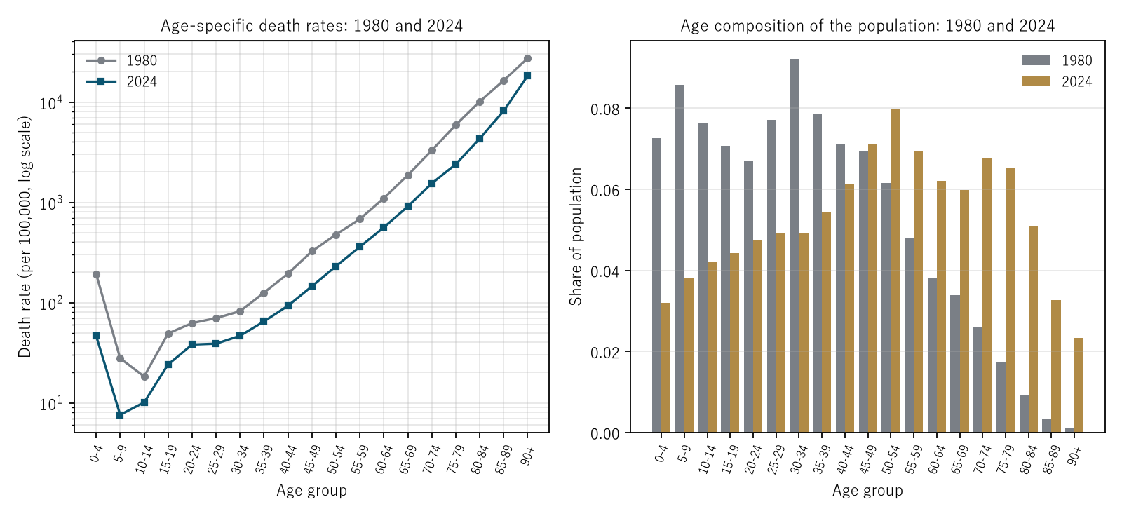
Figure 3: Left, age-specific death rates (log scale); the 2024 line lies below the 1980 line at every age. Right, the age composition of the population; on the high-age side the 2024 bars far exceed the 1980 bars.
5. The Kitagawa decomposition: the age composition pushed up by more than the whole rise
Calculation 5.1 Both sexes, 19 groups, per 100,000
| Interval | Difference | Age-composition effect | Age-specific-rate effect | Composition effect / difference |
|---|---|---|---|---|
| 1980 → 2024 | +713.4 | +1522.3 | −808.8 | 2.134 |
| 1950 → 2024 | +247.3 | +2227.5 | −1980.2 | 9.008 |
| 1950 → 1980 | −466.2 | +323.4 | −789.6 | — |
Observation 5.2: Prediction A holds and Prediction B fails. Against the rise of +713.4 from 1980 to 2024, the age-composition effect is +1522.3, 2.134 times the difference. The age-specific-rate effect is −808.8 and pushes the rise down.
Observation 5.3: From 1950 to 1980 the crude death rate fell by 466.2. Even then the age-composition effect was +323.4, already pushing upward. The rate fell because the age-specific-rate effect of −789.6 outweighed it.
Observation 5.4: The difference from 1950 to 2024 is only +247.3. Its content, however, is a cancellation of +2227.5 and −1980.2. A small difference does not mean a small movement.
Calculation 5.5 Splitting by sex as well as age (38 cells)
| Interval | 19 groups: composition / rate | 38 cells: composition / rate |
|---|---|---|
| 1980 → 2024 | +1522.3 / −808.8 | +1539.5 / −826.4 |
| 1950 → 2024 | +2227.5 / −1980.2 | +2251.3 / −2004.3 |
Observation 5.6: Splitting by sex as well moves the age-composition effect only a little, from +1522.3 to +1539.5. The change in the sex ratio does not move the conclusion.
6. The amount moves with the convention; the direction does not
The Kitagawa decomposition places the weights at the average of the two years. One can also place them at the first year, at the last year, or split interval by interval and add. Each of these reproduces the difference exactly.
Calculation 6.1 Splitting 1980 → 2024 (difference +713.4) in four ways
| Way of splitting | Age-composition effect | Age-specific-rate effect | Composition effect / difference |
|---|---|---|---|
| Kitagawa (average weights) | +1522.3 | −808.8 | 2.134 |
| 1980 weights | +2001.6 | −1288.2 | 2.806 |
| 2024 weights | +1042.9 | −329.5 | 1.462 |
| Summing adjacent intervals | +1218.8 | −505.3 | 1.708 |
Observation 6.2: The age-composition effect moves from +1042.9 to +2001.6; the largest divided by the smallest is 1.919. For 1950 → 2024 it moves from +1173.3 to +3281.8, a factor of 2.797. A figure such as "what fraction is due to aging" depends on the convention of splitting.
Observation 6.3: Yet in all four ways, for both 1980 → 2024 and 1950 → 2024, the order "age-composition effect > difference > 0 > age-specific-rate effect" does not change.
Observation 6.4: The amount is set by convention; the direction is set by the data. What this paper asserts goes as far as the direction.
7. Adjacent years: the three intervals in which the age-specific-rate effect turned positive
Calculation 7.1 Each of the 23 adjacent intervals from 1950 to 2024 is split by the Kitagawa decomposition.
- Intervals with a positive age-composition effect: 23 / 23
- Intervals with a positive age-specific-rate effect: 3 (2020→2021, 2021→2022, 2023→2024)
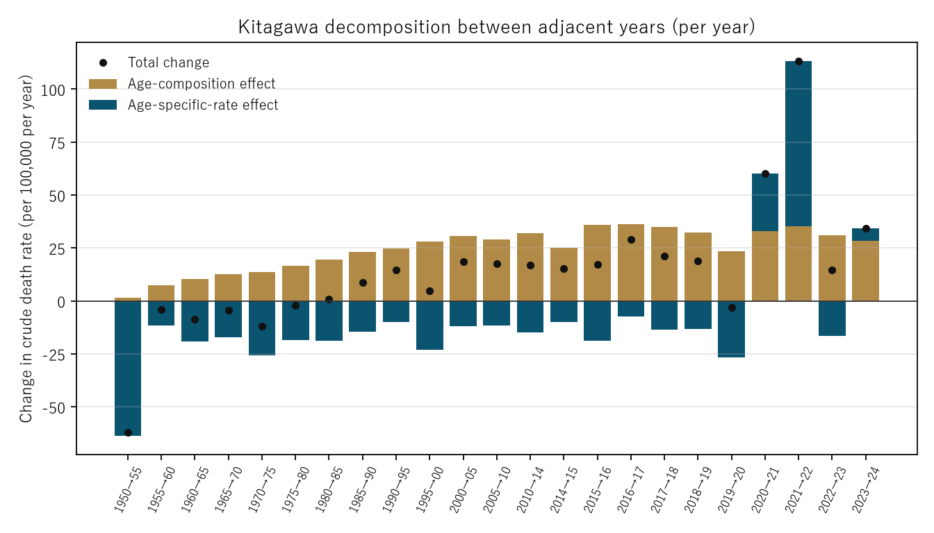
Figure 2: The difference of each interval is divided by the number of years, so the bars are per year. Gold is the age-composition effect, navy is the age-specific-rate effect, and the black dots are the difference of the crude death rate. Where both effects are positive, the navy bar is stacked on the gold one.
Observation 7.2: The age-composition effect per year grew from +1.5 in 1950→1955 to +36.1 in 2016→2017. The upward push of aging has become stronger from interval to interval.
Calculation 7.3 The intervals from 2019 to 2024
| Interval | Difference | Age-composition effect | Age-specific-rate effect |
|---|---|---|---|
| 2019 → 2020 | −3.2 | +23.3 | −26.5 |
| 2020 → 2021 | +60.3 | +33.1 | +27.2 |
| 2021 → 2022 | +113.1 | +35.3 | +77.8 |
| 2022 → 2023 | +14.6 | +31.1 | −16.5 |
| 2023 → 2024 | +34.3 | +28.2 | +6.1 |
Observation 7.4: Splitting 2020 to 2024 as a whole, the difference of +222.3 divides into an age-composition effect of +126.4 and an age-specific-rate effect of +95.9, so the rate side takes 0.432. In the 20 intervals before, the rate effect was always negative. The official age-adjusted death rates also rose, from 13.3 to 14.2 for men and from 7.2 to 7.8 for women.
Observation 7.5: This paper does not state why the age-specific rates rose in these intervals. What the decomposition can say is how much of the rise lies on the side of the rates.
8. Age-adjusted death rates: recomputing the official values
The age-adjusted death rate applies the age-specific rates to one fixed population structure (the standard population) and averages them. The Ministry of Health, Labour and Welfare uses the 2015 model population as the standard (Table 5.2).
Calculation 8.1 Recomputing the official sex-specific values (per 1,000) with the 2015 model population
| Years | Rates in the table | Agree to one decimal | Recomputed − official |
|---|---|---|---|
| 2005–2024 | 90–94 and 95 and over can be split | 26 / 26 | — |
| 1950 | Only a rate for 90 and over | 2 / 2 | men −0.038, women +0.020 |
| 1955–2000 | Only a rate for 90 and over | 0 / 20 | −0.499 to −0.063 |
Calculation 8.2 With the 1985 model population (a standard population that combines ages 85 and over), recomputing the official values of Table 5.2 of the 2016 edition gives agreement to one decimal in 30 of the 32 values, with a largest difference of 0.0937.
Observation 8.3: In the years where ages 95 and over can be split, all official values are reproduced. With the 1985 model (which does not split ages 85 and over), the official values are reproduced including 1955–2000. The discrepancy of the 2015 model in 1955–2000 can therefore be narrowed down to how ages above 90 are split. Which rates the official computation used there has not been checked in this paper. Also, when ages 90 and over are combined and the 2015 model is applied, agreement falls to 7 / 48. Where the standard population splits finely, the rates must not be combined coarsely.
Calculation 8.4 Age-adjusted death rates for both sexes (this paper's computation, 19 groups, per 100,000)
| Year | Crude death rate | 2015 model | 1985 model |
|---|---|---|---|
| 1950 | 1087.6 | 3645.3 | 1631.1 |
| 1980 | 621.4 | 2087.5 | 728.6 |
| 2015 | 1029.8 | 1048.2 | 358.1 |
| 2020 | 1112.5 | 973.8 | 334.4 |
| 2024 | 1334.5 | 1050.3 | 356.7 |
Observation 8.5: The ratio from 1980 to 2024 is 0.503 with the 2015 model and 0.490 with the 1985 model. The levels, however, differ greatly: 2015 model / 1985 model = 2.945 in 2024, 2.865 in 1980 and 2.235 in 1950. The value of an age-adjusted death rate is a product of the convention called the standard population. What should be read is its movement.
Observation 8.6: The total of the 2015 model population, 125,319,000, is close to the sum of the back-calculated population for 2015, 125,321,432. In years close to the standard population, the crude and age-adjusted death rates nearly coincide (1029.8 and 1048.2 in 2015). The two lines change places between 2015 and 2016.
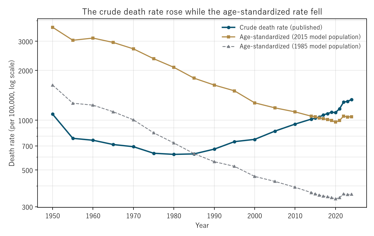
Figure 1: Log scale. Navy is the crude death rate (published), gold is the age adjustment with the 2015 model population, and the grey dashed line is the age adjustment with the 1985 model population (both this paper's computation, both sexes). The two age-adjusted lines differ in level but fall almost in parallel. Both are lowest in 2020.
9. Limitations
- Ages are in five-year groups, with 90 and over combined. Changes in the age distribution within a group enter the age-specific-rate effect.
- Compositions other than age and sex are not measured. Splitting by sex moved the age-composition effect only a little, from +1522.3 to +1539.5, but changes in other compositions, such as region or nationality, are mixed into the age-specific-rate effect.
- The amount of the split moves with the convention (Section 6). What this paper asserts goes only as far as the direction, which does not change across the four ways.
- No cause is stated. Why the age-specific rates fell, and why they rose in the intervals after 2020, lie outside this decomposition. Deaths are not split by cause.
- The denominator is the back-calculated population. In the census years it agrees with the population estimates within 0.00566 in relative terms, but in 2016–2019 the difference widens up to 0.02081.
- The official age-adjusted death rates (2015 model) for 1955–2000 cannot be reproduced from this table alone (Section 8).
- Only Japan and all causes are treated. Nothing is said about other countries, specific causes or regions.
Conclusion
"The death rate rose", once measured, turned out to be the sum of two different movements. From 1980 to 2024 the crude death rate grew by a factor of 2.148. Over the same 44 years the age-specific death rates fell in all 19 groups. In the Kitagawa decomposition, the age-composition effect of +1522.3 pushes up by more than the whole rise, and the age-specific-rate effect of −808.8 pushes down. Changing the way of splitting in four ways moves the amount by a factor of 1.919, but the direction never changes.
What separates them is one thing: whether one moves the age composition or the age-specific rates.
And in the intervals from 2020, the side of the age-specific rates joined the rise for the first time (0.432 for 2020→2024). Its reason lies outside the question this decomposition answers.
Data and reproduction
| Data | Ministry of Health, Labour and Welfare, Vital Statistics 2024 (final data), Volume 1, Tables 5.15 and 5.2 and Appendix Table 6 (2015 and 1985 model populations); 2016 edition, Volume 1, Table 5.2. Statistics Bureau of Japan, Population Estimates, Table 3 (2000–2020). All obtained from e-Stat (accessed 25 September 2026) |
| Terms of use | e-Stat content follows the Government of Japan Standard Terms of Use (Version 2.0), compatible with CC BY 4.0. The numbers in this paper were made by processing these data |
| Coverage | Japan (Japanese nationals in Japan), all causes, 1950–2024 (every five years for 1950–2010, every year for 2014–2024) |
| Age groups | 18 five-year groups and 90 and over (19 in all) |
| Computation | 検算/M001.py (--zu also writes the figures). Every number in the text is taken from 検算/M001_output.txt |
| Raw data | The 6 files as downloaded, with SOURCES.md (URL, date of access, SHA-256), in data/. The computation checks the SHA-256 each time it runs |
| Figures | 図/M001_zu1, 図/M001_zu2, 図/M001_zu3 (png, svg, English versions) |
References
- Kitagawa, E. M. (1955). Components of a Difference Between Two Rates. Journal of the American Statistical Association. 10.1080/01621459.1955.10501299
- Ministry of Health, Labour and Welfare. Vital Statistics 2024 (final data), Volume 1, Tables 5.15 and 5.2 and Appendix Table 6; 2016 edition, Volume 1, Table 5.2 (in Japanese). e-Stat (accessed 25 September 2026). https://www.e-stat.go.jp/
- Statistics Bureau of Japan. Population Estimates, Table 3: Population by Age (Five-Year Groups and 3 Groups) and Sex (as of October 1 of Each Year), Total population, Japanese population (from 2000 to 2020). e-Stat (accessed 25 September 2026). https://www.e-stat.go.jp/
- Yamagishi, Y. (2026). One Table, Two Correct Answers [Paper 183]. Zenodo. 10.5281/zenodo.22104230
- Yamagishi, Y. (2026). The Three Hundredth Census: Whether Two Things Share a Root Is Decidable [Paper 300]. Zenodo. 10.5281/zenodo.22171914
Reference
Yamagishi, Y. (2026). "The Death Rate Rose" Names Two Movements at Once, the Age Composition and the Age-Specific Rates [M001]. Zenodo.
DOI: 10.5281/zenodo.22963112
YOI: https://www.yamagishiyuuki.com/yoi/M001
ORCID: 0009-0006-8587-3450
PDF (English) · PDF (Japanese) · Date proof of the English PDF (OpenTimestamps .ots) · SHA256SUMS
The record page for this paper (in Japanese, with the PDFs in each language and the date proof): YOI M001. This paper is a preprint and has not been peer reviewed.