Abstract
What this paper asks is how far the baseline this series has been using is a valid control — and the answer is: valid for direction, and no control at all for magnitude. No new mathematical theorem and no new law is claimed.
First, for direction the synthetic random walk is a valid control. The autocorrelation of signed returns has a median absolute value of 0.0061 on the measurement and 0.0046 on the random walk, with maxima of only 0.0353 and 0.0125 (Section 3).
Second, and this is the core. ★ Drop the sign and they become different quantities. The autocorrelation of the absolute return has a median of 0.1746 on the measurement and 0.0187 on the random walk. At lag 240 bars — ten days — the measurement still holds 0.1529 (Section 4).
Third, ★ even the 0.0184 left on the random walk is not clustering. Measured on raw absolute differences it is −0.0013. It is a product of taking logs and dividing by the price level, and it is largest for XAUUSD, whose level moved most (max ÷ min = 2.5736) (Section 5).
Fourth, the measurement's clustering is real. On raw differences it is 0.1754, barely different from the 0.1809 of the log version (Section 5).
Fifth, ★ this one difference explains three earlier situations directly. The share of time-outs is 0.3061 against 0.0362, and the ratio of the forward move across ATR quintiles is 2.1064 against 0.9981 (Section 6).
Sixth, ★ so this series' baseline has zero directional information and zero magnitude structure at the same time. The first was intended; the second is a side effect. The three limitations in F027, F028 and F030 all come from this one fact (Section 6).
Scope of this paper: No new mathematical theorem and no new law is claimed — volatility clustering, autocorrelation and random walks are all known. No real course or its proponent is discussed — no real teaching material, author, or vendor is the subject here, and none is named. The subject of this paper is the author's own tool — how far the baseline this series has used is a valid control. Trading is not discussed — no trading performance is measured (Section 7). No mechanism for clustering is offered — why markets cluster is not the question here (Section 7). A correlation over eight points is not evidence of strength — the correlation in Section 6 may be nothing but two separated clumps (Sections 6 and 7). No better baseline is built — how to build a synthetic series with clustering is not treated here (Section 7). The scope is intraday and few instruments — four instruments, six years, one-hour bars. Monthly time-series momentum (dozens of markets, one to twelve month holds) is documented in the academic literature and is not contradicted here. No forecast is claimed.
1. Notation and the question
This series has used a baseline built as a synthetic random walk with independent normal increments down to the movement inside each bar.
| What the baseline was expected to be | What was never checked |
|---|---|
| Free of directional information | Whether it is also free of magnitude structure |
| The same bar count and the same timestamps | How far it differs from the measurement |
| A picture of "what comes out when nothing is there" | Which quantities it is no control for |
Observation 1.1: In F027, F028 and F030 the baseline turned out to be unusable three times. In F027 the synthetic series produced almost no time-outs; in F028 and F030 the layers did not separate magnitude.
Observation 1.2: ★ The same excuse was written all three times: "because there is no volatility clustering". But it was never measured.
Observation 1.3: ★ This paper measures that excuse. Measuring the range of one's own tool is also measurement.
Observation 1.4: The separator is measurement or synthetic random walk. The quantity, the lag, the instrument and the period are all held fixed, and only the series is swapped.
Question: how far is this series' baseline a valid control?
2. State the quantity and the design first
Predictions (written before running)
① The autocorrelation of signed returns is essentially 0 on both. ⇒ For direction, the synthetic random walk is a valid control.
② The autocorrelation of the absolute return is strongly positive and long-lived on the measurement and 0 on the synthetic random walk.
③ So the synthetic random walk is a series with zero directional information and zero magnitude structure at the same time.
④ ★ And that difference should directly explain the three figures seen in F027, F028 and F030.
Design (declared before running and not changed during it)
| Item | Decision |
|---|---|
| Grid | One-hour bars, mid prices, completed bars only |
| Quantities | Log returns and their absolute values |
| Lags | 1, 2, 4, 8, 24, 72, 120, 240 bars |
| Clustering strength | Mean autocorrelation of the absolute return over lags 1, 2, 4, 8, 24 |
| Time-outs | Take-profit = stop-loss = 20 pips, deadline 6 bars (as in F027 and F028) |
| ATR | Ratio of the size of the 24-bar forward move across ATR(14) quintiles (as in F030) |
| Baseline | Synthetic random walk down to within-bar movement (5 series) |
| Instruments | USDJPY, EURUSD, GBPUSD, XAUUSD |
| Period | 2019–2024 |
Observation 2.1: ★ The synthetic series is built by adding differences of constant spread. The per-bar standard deviation is matched to the real data, and the movement inside each bar uses the same spread. ★ Clustering therefore does not exist in it by construction.
Observation 2.2: ★ So this is not a test of whether clustering exists. It is known not to exist on the synthetic side. What this paper measures is how large the difference is.
Observation 2.3: The three figures are re-measured inside this paper. They are not copied from F027, F028 or F030; the same computations are run inside this paper's verification script.
3. Autocorrelation of signed returns — is direction the same?
Calculation 3.1 Autocorrelation by lag (signed returns)
| Lag | USDJPY | EURUSD | GBPUSD | XAUUSD | Measured median | Random median |
|---|---|---|---|---|---|---|
| 1 | −0.0051 | −0.0237 | −0.0353 | −0.0158 | −0.0197 | 0.0005 |
| 2 | 0.0058 | 0.0009 | 0.0060 | 0.0183 | 0.0059 | −0.0046 |
| 8 | 0.0121 | −0.0037 | −0.0047 | −0.0061 | −0.0042 | −0.0043 |
| 24 | −0.0098 | 0.0107 | 0.0072 | 0.0013 | 0.0042 | 0.0020 |
| 120 | 0.0091 | 0.0052 | −0.0143 | −0.0148 | −0.0046 | 0.0041 |
| 240 | 0.0052 | 0.0025 | −0.0035 | 0.0082 | 0.0038 | −0.0061 |
Observation 3.2: Prediction ① held. The median absolute autocorrelation is 0.0061 on the measurement and 0.0046 on the random walk, with maxima of 0.0353 and 0.0125.
Observation 3.3: ★ So for direction the synthetic random walk is a valid control. The measurement side has almost no autocorrelation in the sign either.
Observation 3.4: At lag 1 the measurement is slightly negative, at −0.0197. That is a one-bar reversal, but 0.02 is far smaller than the quantities this series has treated as directional information.
Observation 3.5: ★ That both are zero here is what has supported every baseline in this series so far. Using a synthetic random walk as a control in papers about direction was right.
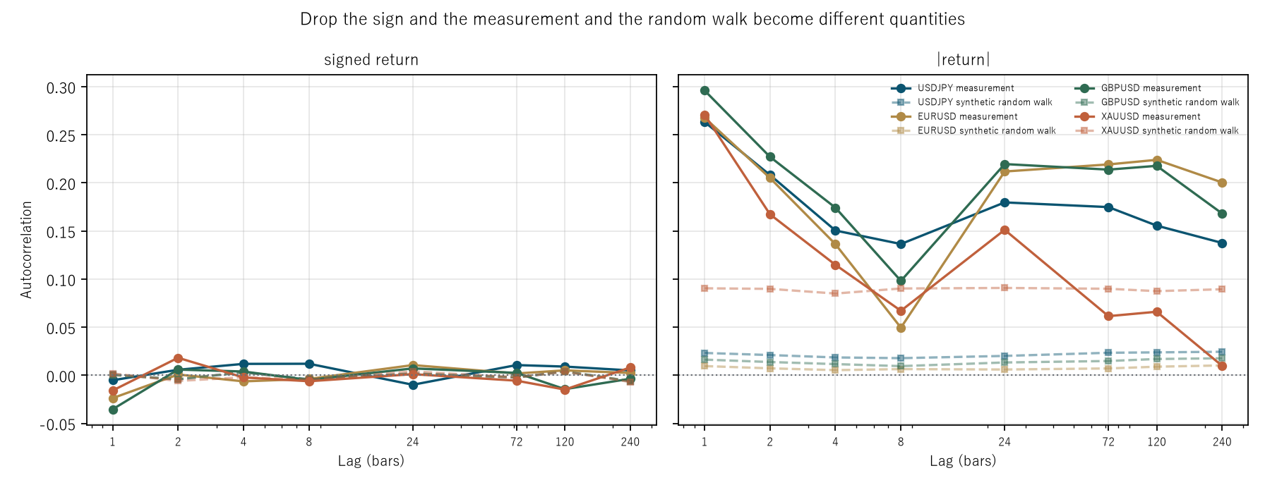
Figure 1: horizontal is the lag (log scale), vertical is the autocorrelation. Left is signed returns, right is the absolute return; solid lines are the measurement and dashed lines the synthetic random walk.
4. Autocorrelation of the absolute return — what about magnitude?
Calculation 4.1 Autocorrelation by lag (absolute return)
| Lag | USDJPY | EURUSD | GBPUSD | XAUUSD | Measured median | Random median | Difference |
|---|---|---|---|---|---|---|---|
| 1 | 0.2634 | 0.2679 | 0.2962 | 0.2710 | 0.2695 | 0.0201 | 0.2493 |
| 2 | 0.2083 | 0.2052 | 0.2271 | 0.1674 | 0.2067 | 0.0178 | 0.1890 |
| 4 | 0.1505 | 0.1363 | 0.1743 | 0.1149 | 0.1434 | 0.0164 | 0.1271 |
| 8 | 0.1365 | 0.0496 | 0.0982 | 0.0671 | 0.0827 | 0.0171 | 0.0655 |
| 24 | 0.1798 | 0.2119 | 0.2196 | 0.1512 | 0.1958 | 0.0197 | 0.1761 |
| 72 | 0.1749 | 0.2192 | 0.2138 | 0.0615 | 0.1944 | 0.0199 | 0.1745 |
| 120 | 0.1556 | 0.2240 | 0.2178 | 0.0661 | 0.1867 | 0.0180 | 0.1687 |
| 240 | 0.1376 | 0.2005 | 0.1682 | 0.0099 | 0.1529 | 0.0237 | 0.1292 |
Observation 4.2: ★ This is the core. On the same series, with nothing changed but dropping the sign, the measurement gives a median of 0.1746 and the random walk 0.0187.
Observation 4.3: ★ And the measurement is long-lived. At lag 240 bars — ten days — it still holds 0.1529. It dips to 0.0827 at lag 8 and returns to 0.1958 at lag 24. That reads as a daily cycle, but this paper does not measure it.
Observation 4.4: The clustering strength (the mean over lags 1, 2, 4, 8 and 24) is 0.1809 on the measurement and 0.0184 on the random walk. ★ Nearly tenfold.
Observation 4.5: Only XAUUSD falls away at long lags, to 0.0099 at lag 240, while the other three hold 0.1376 to 0.2005. ★ Gold's clustering may be shorter, but this paper does not investigate the mechanism.
Observation 4.6: The random walk's range is wide too, from −0.0099 to 0.2248. Its median is 0.0187, not zero. ★ Clustering should not exist there by construction, so the next section chases this down.
5. Where does the remainder on the random walk come from?
Calculation 5.1 Measured on log returns and on raw differences
| Instrument | Clustering of the absolute return | Clustering of the raw difference | Price max ÷ min | |
|---|---|---|---|---|
| USDJPY | measured | 0.1877 | 0.2056 | 1.5866 |
| USDJPY | random | 0.0215 | −0.0013 | 1.6153 |
| EURUSD | measured | 0.1742 | 0.1644 | 1.2936 |
| EURUSD | random | 0.0070 | −0.0013 | 1.3766 |
| GBPUSD | measured | 0.2031 | 0.1861 | 1.3691 |
| GBPUSD | random | 0.0146 | −0.0013 | 1.5078 |
| XAUUSD | measured | 0.1543 | 0.1646 | 2.1997 |
| XAUUSD | random | 0.0893 | −0.0011 | 2.5736 |
Observation 5.2: ★ On raw differences the random walk's clustering vanishes, to a median of −0.0013. ★ Exactly as built: none at all.
Observation 5.3: ★ So the 0.0184 left on the random walk is not clustering. It is a product of taking logs and dividing by the price level. When the level drifts slowly, the same size of difference gives a log return that stretches and shrinks.
Observation 5.4: ★ And it is largest for the instrument whose level moved most. XAUUSD's random walk has a price max ÷ min of 2.5736, the largest of the four, and the largest clustering at 0.0893. EURUSD is 1.3766 and 0.0070.
Observation 5.5: ★ The measurement's clustering, meanwhile, is real. On raw differences it is 0.1754, barely different from the 0.1809 of the log version. Changing the divisor does not remove it.
Observation 5.6: This is a shape this series has met before. Normalizing is not neutral. ★ Taking a logarithm — an ordinary operation — manufactured a pattern up to 0.0893 where none existed.
6. Re-measuring the three situations inside this paper
Calculation 6.1 Time-outs and the ATR quintile ratio
| Instrument | Share of time-outs | ATR quintile ratio | Clustering strength | |
|---|---|---|---|---|
| USDJPY | measured | 0.3538 | 3.3143 | 0.1877 |
| USDJPY | random | 0.0340 | 0.9981 | 0.0215 |
| EURUSD | measured | 0.4561 | 1.9352 | 0.1742 |
| EURUSD | random | 0.2154 | 0.9980 | 0.0070 |
| GBPUSD | measured | 0.2584 | 1.8978 | 0.2031 |
| GBPUSD | random | 0.0373 | 0.9981 | 0.0146 |
| XAUUSD | measured | 0.0203 | 2.2776 | 0.1543 |
| XAUUSD | random | 0.0000 | 0.9941 | 0.0893 |
Observation 6.2: ★ The ATR quintile ratio is the clearest. The measurement has a median of 2.1064 and the random walk 0.9981. On the random walk all four instruments fall between 0.9941 and 0.9981 — that is, 1.
Observation 6.3: ★ This is exactly what F030 measured. The distinction between a high-ATR stretch and a low-ATR stretch does not exist in the synthetic series. Built at constant spread, it could not.
Observation 6.4: The share of time-outs is a median of 0.3061 on the measurement and 0.0362 on the random walk. But the ranges are wide: 0.0203 to 0.4561 and 0.0000 to 0.2154.
Observation 6.5: XAUUSD's measurement has only 0.0203 time-outs, because the barriers are fixed in pips and an instrument that moves a lot reaches them easily. ★ Time-outs are not decided by clustering alone.
Observation 6.6: The correlation with clustering strength is +0.5682 for time-outs and +0.8102 for the ATR quintile ratio. With only eight points, the value itself is not evidence of strength. ★ And it may be nothing but two separated clumps. This paper does not use it as evidence of a relation.
Observation 6.7: ★ What this paper can say is that the two clumps are clearly apart: 0.0184 against 0.1809 in clustering strength, and 0.9981 against 2.1064 in the ATR quintile ratio.
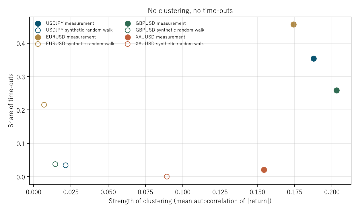
Figure 2: horizontal is the clustering strength, vertical is the share of time-outs. Filled markers are the measurement, open markers the synthetic random walk.
7. Limitations
- No mechanism for clustering is offered. Why markets cluster is not the question here.
- No better baseline is built. How to build a synthetic series with clustering is not treated. What this paper did was measure the range of the present tool.
- A correlation over eight points is not evidence of strength. The correlation in Section 6 may be nothing but two separated clumps.
- Time-outs are not decided by clustering alone. The barriers are fixed in pips, so an instrument that moves a lot reaches them easily.
- XAUUSD's fall at long lags is not investigated. Why it reaches 0.0099 at lag 240 is not measured.
- The dip at lag 8 and the return at lag 24 are not investigated. They read as a daily cycle, but that is not measured.
- One-hour bars are fixed. Clustering looks different on other bar sizes.
- Four instruments over six years. Nothing is said about other markets or other periods.
Conclusion
This series has used a baseline built as a synthetic random walk with independent normal increments down to the movement inside each bar. In F027, F028 and F030 it turned out to be unusable three times, and the same excuse was written all three times: "because there is no volatility clustering". This paper measured that excuse.
For direction the synthetic random walk is a valid control. The autocorrelation of signed returns has a median absolute value of 0.0061 on the measurement and 0.0046 on the random walk, with maxima of 0.0353 and 0.0125. ★ Using it as a control in papers about direction was right.
★ But drop the sign and they become different quantities. The autocorrelation of the absolute return has a median of 0.1746 on the measurement and 0.0187 on the random walk, and at lag 240 bars — ten days — the measurement still holds 0.1529. The clustering strength is 0.1809 against 0.0184, nearly tenfold.
★ And even that 0.0184 on the random walk is not clustering. On raw absolute differences it is −0.0013, exactly as built: none at all. What remained was a product of taking logs and dividing by the price level, and it is largest for XAUUSD, whose level moved most (max ÷ min = 2.5736), at 0.0893. Normalizing is not neutral. Taking a logarithm — an ordinary operation — manufactured a pattern where none existed.
The measurement's clustering, by contrast, is real: 0.1754 on raw differences against 0.1809 on logs.
★ This one difference explains three earlier situations directly. The ratio of the forward move across ATR quintiles is 2.1064 on the measurement while all four random-walk instruments fall between 0.9941 and 0.9981 — that is, 1. The share of time-outs is 0.3061 against 0.0362.
★ So this series' baseline has zero directional information and zero magnitude structure at the same time. The first was intended; the second is a side effect.
So before using the baseline, one must see whether the quantity being measured is on the direction side or the magnitude side. ★ And this paper builds no better baseline. What it did was measure the range of the present tool.
Data and reproduction
| Data | FX is Dukascopy-derived tick data (from 2019 onward, confirmed identical down to the millisecond, bid and ask). Gold is Dukascopy |
| Period | 2019–2024 (six years) |
| Instruments | USDJPY, EURUSD, GBPUSD, XAUUSD |
| Bars | One-hour bars, mid prices, closes of completed bars only. No bar is made where there are no ticks |
| Quantities | Log returns and their absolute values, and raw absolute differences |
| Lags | 1, 2, 4, 8, 24, 72, 120, 240 bars |
| Three situations | Time-outs (take-profit = stop-loss = 20 pips, deadline 6 bars) / ratio of the 24-bar forward move across ATR(14) quintiles |
| Baseline | Synthetic random walk down to within-bar movement (5 series), built by adding differences of constant spread |
| Verification | 検算/F033.py (--zu also writes the figures). Every figure in the text comes from 検算/F033_output.txt |
| Figures | 図/F033_zu1, 図/F033_zu2 (png, svg, English versions) |
| Random seeds | Fixed. Re-running gives the same values |
| Foundation check | _ツール/audit_bars.py (bar look-ahead, daylight saving, day boundaries). The record is _土台の検査.txt |
References
- Yamagishi, Y. (2026). Where You Put the Time-Outs Decides the Share of "Both Lose" [F027]. Zenodo. 10.5281/zenodo.22892724
- Yamagishi, Y. (2026). The Distance to the Level Ahead Moves the Time-Outs, Not the Win Rate [F028]. Zenodo. 10.5281/zenodo.22892891
- Yamagishi, Y. (2026). Layering on a Magnitude Does Not Produce a Direction [F030]. Zenodo. 10.5281/zenodo.22893420
Reference
Yamagishi, Y. (2026). A Synthetic Random Walk Has No Volatility Clustering [F033]. Zenodo.
DOI: 10.5281/zenodo.22893674
YOI: https://www.yamagishiyuuki.com/yoi/F033
ORCID: 0009-0006-8587-3450
PDF (English) · PDF (Japanese) · Date proof of the English PDF (OpenTimestamps .ots) · SHA256SUMS
The record page for this paper (in Japanese, with the PDFs in each language and the date proof): YOI F033. This paper is a preprint and has not been peer reviewed.