Abstract
What this paper asks is what actually sets the reduction in risk behind "split across several currency pairs and the risk goes down". No new mathematical theorem and no new law is claimed.
First, ★ the pair correlations are all over the place. EURUSD with GBPUSD is +0.6577 and USDJPY with EURUSD is −0.4252; the six pairs land on both sides of zero (Section 3).
Second, and this is the core of the paper: ★★ averaging them gives +0.0455, which looks almost independent. The effective count is 3.5194, or 0.8799 of the 4 streams. "An effective count near 4" does not mean "the four were independent" (Section 4).
Third, ★★ split two at a time, the same "split in two" opens from 1.2065 to 3.4797. EURUSD with GBPUSD gives 1.2065 — barely one stream's worth (Section 5).
Fourth, ★ the correlations move year by year, and one pair keeps climbing. EURUSD with GBPUSD goes from +0.5152 in 2020 to +0.8009 in 2023, while the effective count falls from 4.2227 to 3.3299 (Section 6).
Fifth, ★ prediction ⑤ failed. The maximum drawdown shrank by 2.2229, better than volatility's 1.8760 (Section 7).
Sixth, ★ splitting by hour of the day is closer to independent than splitting by instrument. Effective count ÷ streams is 0.8799 for instruments against 1.0008 for hours. Those are different hours of the same day, however, not independent trades (Section 7).
Scope of this paper: no new mathematical theorem and no new law is claimed — the variance of an equally weighted book is an elementary result. No real course, author, or vendor is the subject here, and none is named. No trading is discussed — neither performance nor profit and loss is measured, and no advice on how to split is given. Predictions ②③⑤ failed — ② put the effective count far too low (Sections 4, 6 and 7). The hour-of-day streams are not independent trades — they are different hours of the same day (Section 7). Four instruments are fixed (Section 7). The scope is intraday and few instruments — four instruments over six years. Results documented at longer holding periods, such as monthly time-series momentum, are not contradicted. No prediction is claimed.
1. Notation and the question
"Split across several currency pairs and the risk goes down," people say — usually meaning that four streams give a quarter of the risk.
Split equally n ways, the book's variance is (1/n)·σ²·(1 + (n−1)·ρ). So:
effective count = n ÷ ( 1 + (n−1)·ρ )
| What gets said | What does not get said |
|---|---|
| Four streams, so a quarter | How correlated those four were |
| I am diversified | The count is yours to choose; the correlation is not |
| The correlation is low | Low on average, or low in every pair? |
Observation 1.1: ★ At ρ = 0 it is n streams' worth, at ρ = 1 one stream's worth. What does the work is the correlation, not the count.
Observation 1.2: ★ And the correlation is not yours to choose. You can set the number of streams; you cannot set how much the market moves together.
Observation 1.3: The separator here is the correlation between the pair. The instruments, the period, the grid and the way returns are taken are all held fixed, and what is looked at is not how many streams there were but how correlated they were.
Question: in actual foreign exchange, what is that correlation?
2. State the quantities and the design first
Declared before the run and unchanged during it.
| Grid | 1-hour bars (mid price, completed bars only) |
| Returns | Every 24 bars, non-overlapping, in pips |
| Alignment | ★ The bar timestamps are aligned first, then cut into 24s |
| Correlation | Pearson |
| Effective count | n ÷ (1 + (n−1)·ρ̄) (formula) and σ²(one stream) ÷ σ²(book) (measured) |
| Book | Equally weighted. Instruments are scaled to equal volatility |
| Windows | Calendar years 2019–2024 / hours UTC 0-7, 8-15, 16-23 |
| Baseline | Synthetic random walk down to within the bar (3 draws, an independent seed per instrument) |
| Separator | The correlation between the pair (not how many streams) |
| Instruments and period | USDJPY, EURUSD, GBPUSD, XAUUSD / 2019–2024 |
Observation 2.1: ★ The order of the alignment is the point. The instruments do not share the same set of bars, so cutting into 24s first leaves the boundaries out of step. Cutting first made every correlation NaN.
Observation 2.2: Returns are taken every 24 bars, leaving 1,395 aligned points. The volatilities are 78.3978 for USDJPY, 48.5303 for EURUSD, 72.6165 for GBPUSD and 178.4380 pips for XAUUSD. ★ The hourly series hold 36,534, 36,554, 36,535 and 34,892 bars, so the aligned points are fewer than any single instrument's.
Observation 2.3: ★ That the interval at which returns are measured moves the Sharpe ratio was measured in [F032]. This paper fixes that interval at 24 bars and does not move it.
Predictions (written before measuring)
① Pairs sharing a currency are highly correlated, so the effective count does not grow.
② ★ Split equally across four instruments, the effective count is not 4 but around 2.
③ ★★ The correlation moves over time; measured window by window, the effective count changes a great deal.
④ A synthetic random walk (built independently) gives an effective count equal to the number of streams.
⑤ ★ The maximum drawdown shrinks worse than the variance does.
⑥ ★ Splitting by hour of the day is less correlated than splitting by instrument.
3. The pair correlations run from −0.4252 to +0.6577
Calculation 3.1 The six pairs
| Pair | Correlation |
|---|---|
| EURUSD with GBPUSD | +0.6577 |
| USDJPY with EURUSD | −0.4252 |
| EURUSD with XAUUSD | +0.3797 |
| USDJPY with XAUUSD | −0.3325 |
| USDJPY with GBPUSD | −0.3284 |
| GBPUSD with XAUUSD | +0.3218 |
Observation 3.2: Prediction ① held. ★ The highest is EURUSD with GBPUSD at +0.6577, a pair with the dollar on the same side in both.
Observation 3.3: ★ All three pairs containing USDJPY are negative (−0.4252, −0.3325, −0.3284), because the dollar sits on the other side.
Observation 3.4: ★★ Three positive, three negative — and of similar size. That is what matters in the next section.
4. Averaged, they cancel, and the effective count comes out at 3.5194
Calculation 4.1 Split equally four ways
| Quantity | Value |
|---|---|
| Streams n | 4 |
| Mean pair correlation ρ̄ | +0.0455 |
| Effective count (formula n ÷ (1+(n−1)ρ̄)) | 3.5194 |
| Effective count (measured σ²(one) ÷ σ²(book)) | 3.5194 |
| Difference between formula and measurement | 0.000000 |
Observation 4.2: ★★ Prediction ② failed. The effective count is not around 2 but 3.5194. That is 0.8799 of the 4 streams — far closer to 4 than I expected.
Observation 4.3: ★★ The reason is cancellation. +0.6577 and −0.4252 mix, and the average comes out at +0.0455.
Observation 4.4: ★★ So "an effective count near 4" does not mean "the four were independent". There is a +0.6577 pair inside. A low average and a low correlation in every pair are different things.
Observation 4.5: The formula and the measurement agree exactly (difference 0.000000). ★ That is a check, not a finding. It merely confirms that an equally weighted book's variance is (1/n)·σ²·(1+(n−1)ρ).
Observation 4.6: Risk (volatility) shrinks by √3.5194 = 1.8760. ★ Split four ways, it does not halve.
5. Split two at a time, it opens from 1.2065 to 3.4797
Calculation 5.1 The effective count of each pair
| Pair | Correlation | Effective count |
|---|---|---|
| USDJPY with EURUSD | −0.4252 | 3.4797 |
| USDJPY with XAUUSD | −0.3325 | 2.9961 |
| USDJPY with GBPUSD | −0.3284 | 2.9780 |
| GBPUSD with XAUUSD | +0.3218 | 1.5130 |
| EURUSD with XAUUSD | +0.3797 | 1.4496 |
| EURUSD with GBPUSD | +0.6577 | 1.2065 |
Observation 5.2: ★★ The same "split in two" opens from 1.2065 to 3.4797. The median is 2.2455.
Observation 5.3: ★★ EURUSD with GBPUSD gives 1.2065 — barely one stream's worth. Two positions are on, and the risk falls by only √1.2065.
Observation 5.4: ★★ Negatively correlated pairs, on the other hand, exceed 2. USDJPY with EURUSD gives 3.4797. Split in two, it works like three and a half.
Observation 5.5: ★ So "how many I split it into" says nothing about the effective count. The same 2 reads as 1.2065 or as 3.4797.
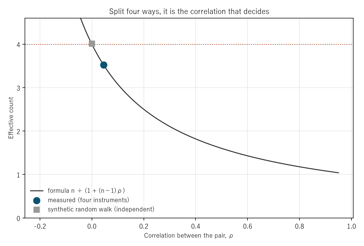
Figure 1: the pair correlation ρ on the horizontal axis and the effective count on the vertical. The curve is the formula n ÷ (1 + (n−1)ρ), and the points are the measurement and the random walk.
6. The correlations move year by year, and one pair keeps climbing
Calculation 6.1 By calendar year
| Year | Mean pair correlation | Effective count | Highest pair |
|---|---|---|---|
| 2019 | −0.0176 | 4.2227 | USDJPY/XAUUSD −0.5660 |
| 2020 | +0.0159 | 3.8181 | EURUSD/GBPUSD +0.5152 |
| 2021 | +0.0603 | 3.3871 | EURUSD/GBPUSD +0.6840 |
| 2022 | +0.0530 | 3.4514 | EURUSD/GBPUSD +0.7524 |
| 2023 | +0.0437 | 3.5367 | EURUSD/GBPUSD +0.8009 |
| 2024 | +0.0671 | 3.3299 | EURUSD/GBPUSD +0.7663 |
Observation 6.2: ★ Prediction ③ failed. The effective count runs from 4.2227 to 3.3299, a maximum ÷ minimum of only 1.2681. I wrote "changes a great deal", and it does not.
Observation 6.3: ★★ The contents move, though. EURUSD with GBPUSD climbs from +0.5152 in 2020 to +0.8009 in 2023. The average stays put because the other pairs move the other way and cancel it.
Observation 6.4: ★ 2019 is the one year whose highest pair is USDJPY with XAUUSD at −0.5660. That year the average is −0.0176 and the effective count reaches 4.2227, above 4.
Observation 6.5: ★ Watching only the average, you would not notice a +0.8009 pair growing. That is the same shape as Section 4.
7. The tail, the hours, the baseline and limitations
Calculation 7.1 How the maximum drawdown shrinks
| Quantity | Value |
|---|---|
| Maximum drawdown of one stream (median) | 38.8708 |
| Maximum drawdown of the four combined | 17.4867 |
| Shrink factor | 2.2229 |
| Volatility's shrink, √effective count | 1.8760 |
| Tail ÷ volatility | 1.1849 |
Observation 7.2: ★ Prediction ⑤ failed. The tail shrank better (2.2229 against 1.8760, a ratio of 1.1849). ★ That the maximum drawdown belongs to the order of the trades was measured in [F031], however, so this single number should not be read hard.
Calculation 7.3 Splitting by instrument or by hour
| Split by | Streams | Mean pair correlation | Effective count | Effective ÷ streams |
|---|---|---|---|---|
| Instrument (four) | 4 | +0.0455 | 3.5194 | 0.8799 |
| Hour of the day (three) | 3 | −0.0004 | 3.0023 | 1.0008 |
Observation 7.4: Prediction ⑥ held. The three hour-block correlations are −0.0002, −0.0008 and −0.0002 — essentially zero.
Observation 7.5: Those are different hours of the same day, however. They are not independent trades.
Calculation 7.6 The baseline (synthetic random walk, independent per instrument)
| Seed | Mean pair correlation | Effective count (formula) | Effective count (measured) |
|---|---|---|---|
| 0 | −0.0018 | 4.0213 | 4.0213 |
| 1 | −0.0011 | 4.0129 | 4.0129 |
| 2 | +0.0005 | 3.9941 | 3.9941 |
Observation 7.7: Prediction ④ held. The median is 4.0129, matching the 4 streams. ★ That too is a check, not a finding.
Observation 7.8: ★ The measured 3.5194 is 0.8770 of it. So the four instruments do the work of 0.8770 of four independent streams.
Observation 7.9: ★ What this baseline is zero about was measured in [F033].
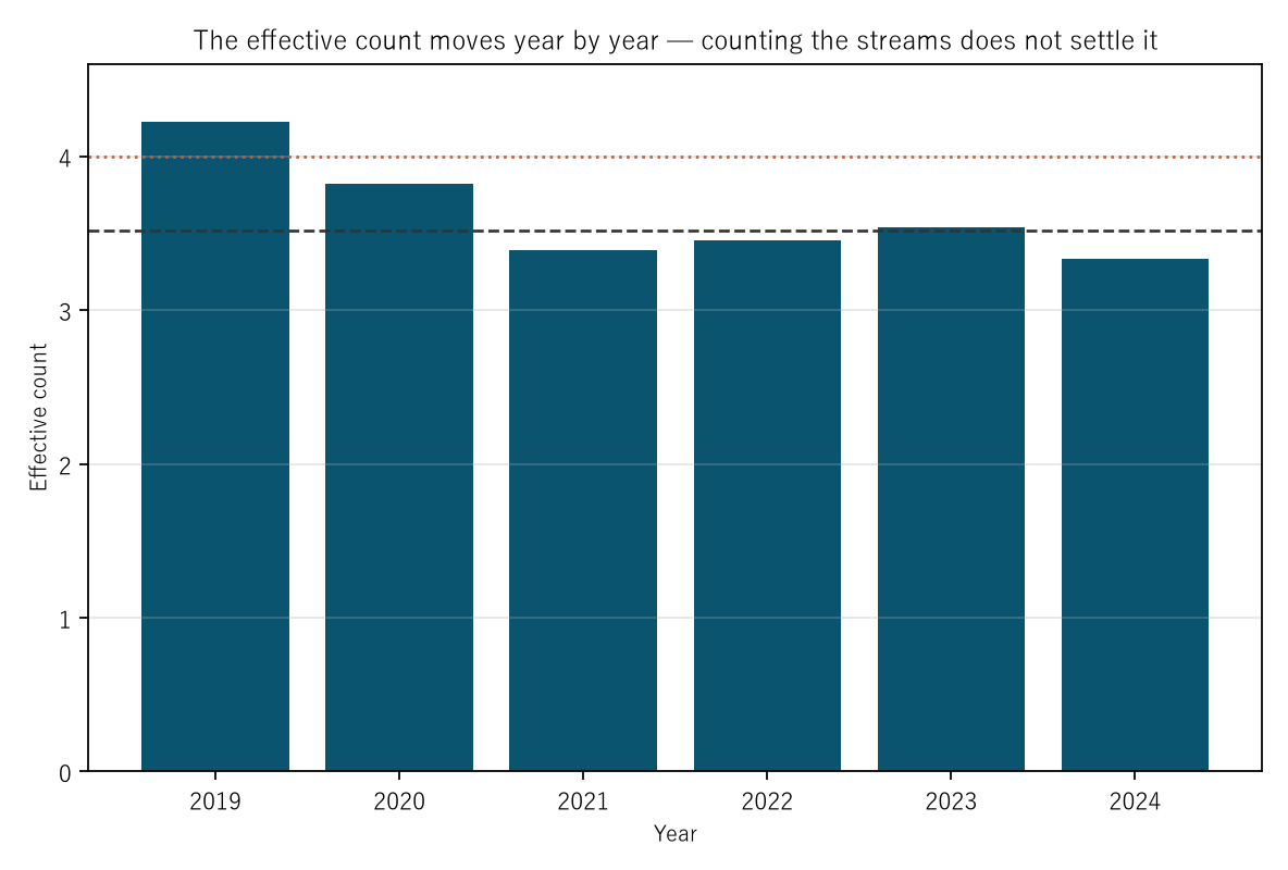
Figure 2: year on the horizontal axis and the effective count on the vertical. The dotted line is the 4 streams and the dashed line the 3.5194 of the whole period.
Limitations
- Prediction ② was badly wrong. I put the effective count at around 2; it is 3.5194. I had not thought about the cancellation.
- Predictions ③ and ⑤ failed too. ③ overstated the year-to-year movement and ⑤ got the tail's shrinking backwards.
- The hour-of-day streams are not independent trades. They are different hours of the same day.
- Four instruments are fixed. A different set gives a different average.
- The return interval is fixed at 24 bars.
- No trading is discussed. Neither performance nor profit and loss is measured, and no advice on how to split is given.
- Four instruments, six years. Nothing is claimed about other markets or other periods.
Conclusion
When someone says "four ways, so a quarter", what is being counted is the number of streams. But what the formula contains is the correlation.
★ The six pair correlations ran from +0.6577 to −0.4252. Three positive, three negative, and of similar size.
★★ So averaged they give +0.0455 and look almost independent. The effective count is 3.5194, 0.8799 of the 4 streams. I predicted around 2 and was wrong.
★★ But "an effective count near 4" does not mean "the four were independent". There is a +0.6577 pair inside. A low average and a low correlation in every pair are different things.
★★ Split two at a time, that shows plainly. The same "split in two" opens from 1.2065 to 3.4797. EURUSD with GBPUSD gives 1.2065, barely one stream's worth; USDJPY with EURUSD gives 3.4797, three and a half.
★ Year by year the average barely moves (4.2227 to 3.3299, a factor of 1.2681), while EURUSD with GBPUSD climbs from +0.5152 to +0.8009. Watching only the average, you would not notice the pair that is growing.
★ Three of six predictions failed. ② put the effective count too low, ③ overstated the year-to-year movement and ⑤ got the tail backwards — it shrank better (2.2229 against 1.8760).
So what should be written down when claiming diversification is not the number of streams. ★ It is the list of pair correlations, their average, and the highest one. The average is what cancellation leaves behind, and by itself it does not show what is inside.
Data and reproduction
| Data | Foreign exchange from Dukascopy-derived ticks (from 2019 onward, matching to the millisecond, bid and ask, has been verified). Gold from Dukascopy |
| Period | 2019–2024 (six years) |
| Instruments | USDJPY, EURUSD, GBPUSD, XAUUSD |
| Bars | 1-hour, mid price, completed bars only. Bars with no ticks are not created |
| Returns | Every 24 bars, non-overlapping, in pips |
| Alignment | The bar timestamps are aligned across the four instruments first, then cut into 24s |
| Effective count | n ÷ (1 + (n−1)·ρ̄) (formula) and σ²(one stream) ÷ σ²(book) (measured); ρ̄ is the mean pair correlation |
| Book | Equally weighted. Instruments are scaled to equal volatility |
| Windows | Calendar years 2019–2024 / hours UTC 0-7, 8-15, 16-23 |
| Baseline | Synthetic random walk down to within the bar (3 draws), with an independent seed per instrument |
| Verification | 検算/F048.py (--zu also writes the figures). Every number in the text comes from 検算/F048_output.txt |
| Figures | 図/F048_zu1, 図/F048_zu2 (png, svg, English versions) |
| Random seeds | Fixed. Re-running gives the same values |
| Substrate check | _ツール/audit_bars.py (bar look-ahead, daylight saving, day boundary). The record is _土台の検査.txt |
References
- Yamagishi, Y. (2026). The Maximum Drawdown Belongs to the Order of the Trades [F031]. Zenodo. 10.5281/zenodo.22893510
- Yamagishi, Y. (2026). The Sharpe Ratio Belongs to the Interval You Measured It On [F032]. Zenodo. 10.5281/zenodo.22893620
- Yamagishi, Y. (2026). A Synthetic Random Walk Has No Volatility Clustering [F033]. Zenodo. 10.5281/zenodo.22893674
Reference
Yamagishi, Y. (2026). The Effective Count of a Diversified Book Is What Is Left After the Pair Correlations Cancel [F048]. Zenodo.
DOI: 10.5281/zenodo.22896842
YOI: https://www.yamagishiyuuki.com/yoi/F048
ORCID: 0009-0006-8587-3450
PDF (English) · PDF (Japanese) · Date proof of the English PDF (OpenTimestamps .ots) · SHA256SUMS
The record page for this paper (in Japanese, with the PDFs in each language and the date proof): YOI F048. This paper is a preprint and has not been peer reviewed.