Abstract
What this paper asks is where the after-the-fact step enters "range → counter-trend, trend → trend" — and the answer is: not in the judgement window but in how the assignment is decided. No new mathematical theorem and no new law is claimed.
First, switching the judgement window to the forward one does not enlarge the effect as much as expected. The end-to-end spread across layers goes from 1.7225 to 3.7407 pips at n=24 (2.2 times), and at n=6 it narrows from 1.2673 to 0.3444 pips (0.3 times) (Section 4).
Second, ★ the reason is that the efficiency ratio is a magnitude. It measures "how straight the move was" and says nothing about which way. So only magnitude leaks (Section 4).
Third, prediction ② failed. It said "with a past window both vanish", but the layer effect survives on the past window (+1.2673 at n=6, +1.7225 pips at n=24) (Section 3).
Fourth, prediction ③ failed too. The random walk's forward version has end-to-end spreads of −0.2048 (n=6) and −1.7516 pips (n=24), the opposite sign to the measurement. "The random walk gives just as much" cannot be said (Section 6).
Fifth, and this is the core. ★ So another after-the-fact step was measured (added afterwards). Taking whichever of trend-following and counter-trend did better in each layer is just |D|. Even on a synthetic random walk with zero directional information, |D| is above zero in all 20 layers (median 0.5544 pips, against 0.7050 on the measurement) (Section 5.5).
Sixth, ★ prediction ④ held. The multiple for the forward version is 0.3 at n=6 and 2.2 at n=24 — the longer the window, the larger (Section 5).
Scope of this paper: No new mathematical theorem and no new law is claimed — the efficiency ratio, look-ahead, selection bias and random walks are all known. No real course or its proponent is discussed — no real teaching material, author, or vendor is the subject here, and none is named. Trading is not discussed — no costs are included, so the figures here are not trading performance (Section 7). Calculation 5.5 was added afterwards — it was measured once it became clear that only magnitude leaks, so it is after the fact (Section 5.5). The layer cuts use the whole period — the quintile boundaries come from the whole sample, which is itself a mild look-ahead; but both versions are cut the same way, so the comparison is fair (Sections 2 and 7). The overlap is not removed — measurements are taken on every bar, so the observations overlap (Section 7). D and the daily t disagree in sign in some layers — days with many observations are making the overall mean, and both are printed here (Section 3). The scope is intraday and few instruments — four instruments, six years, one-hour bars. Monthly time-series momentum (dozens of markets, one to twelve month holds) is documented in the academic literature and is not contradicted here. No forecast is claimed.
1. Notation and the question
It is often said that "in a range you fade, in a trend you follow".
| What gets said | What does not |
|---|---|
| Fade in a range | When the regime was judged |
| Follow in a trend | When it was decided which layer gets which |
| So telling them apart is what matters | Whether a series with no edge gives the same shape |
Observation 1.1: ★ There are two places an after-the-fact step can enter: the judgement window (is the regime being decided from the move that is still to come?) and how the assignment is decided (was which layer gets which chosen after seeing the results?).
Observation 1.2: The separator is which window judged the regime. The formula and the layer cuts are held identical and only the window is swapped between past and forward.
Observation 1.3: The regime is measured by the efficiency ratio: end-to-end distance ÷ path length, so closer to 1 means the move was straighter (a trend).
Observation 1.4: ★ The efficiency ratio is a magnitude. Built from absolute values, it contains no direction. That property matters later.
Question: where does the after-the-fact step enter "range → counter-trend, trend → trend"?
2. State the quantity and the design first
Predictions (written before running)
① With a look-ahead judgement, trend-following wins a lot in the trend layer and loses a lot in the range layer.
② With a past judgement, both largely vanish.
③ ★ A synthetic random walk with zero directional information gives just as much under the look-ahead version.
④ The look-ahead effect grows with the window length.
Design (declared before running and not changed during it)
| Item | Decision |
|---|---|
| Grid | One-hour bars, mid prices, completed bars only |
| Window | n = 6 and 24 bars |
| Regime | Efficiency ratio = end-to-end ÷ path length |
| Past version … from i−n to i (known at entry) | |
| Forward version … from i to i+n (not known at entry) | |
| Layers | 5 quintiles of the efficiency ratio (cut within the same instrument and period) |
| Signal | Trend-following = sign(c[i] − c[i−n]); counter-trend is its negation |
| Horizon | The change over the next n bars (pips) |
| Measured | D = mean of the signed return / daily-clustered t |
| Baseline | Synthetic random walk down to within-bar movement (3 series) |
| Instruments | USDJPY, EURUSD, GBPUSD, XAUUSD |
| Period | 2019–2024 |
Observation 2.1: ★ The two versions differ only in the direction of the window. The formula, the number of layers, the signal and the horizon are identical.
Observation 2.2: The quintile boundaries come from the whole period, which is itself a mild look-ahead. But both versions are cut the same way, so the comparison between them is fair.
Observation 2.3: The forward version is a quantity that cannot be computed at entry. This paper builds it deliberately to see what happens.
The bar counts are 36,534, 36,554, 36,535 and 34,892.
3. Judging the regime on the past window
Calculation 3.1 D of trend-following by efficiency-ratio quintile (medians across four instruments)
| Window | Layer | Median ER | Count | D of trend-following | Daily t |
|---|---|---|---|---|---|
| 6 | 1 (range) | 0.0754 | 7,298 | −0.5990 | 0.13 |
| 6 | 3 | 0.3878 | 7,298 | −0.2195 | 0.59 |
| 6 | 5 (trend) | 0.8292 | 7,298 | 0.6684 | −4.97 |
| 24 | 1 (range) | 0.0369 | 7,296 | 0.2614 | 1.55 |
| 24 | 2 | 0.1134 | 7,295 | 1.5086 | 1.95 |
| 24 | 3 | 0.1975 | 7,296 | 1.5576 | 1.89 |
| 24 | 4 | 0.3009 | 7,295 | 2.1346 | 0.32 |
| 24 | 5 (trend) | 0.4618 | 7,296 | 1.9839 | −3.20 |
Observation 3.2: Prediction ② failed. It said "with a past window both largely vanish", but the layer effect survives: end to end it is +1.2673 at n=6 and +1.7225 pips at n=24.
Observation 3.3: The daily t reaches 2 in absolute value in 14 of 40 layers. Chance would give about 2, so the layers are separating something.
Observation 3.4: ★ But D and the daily t disagree in sign in some layers. At n=6, layer 5 has D +0.6684 against t −4.97. ★ Days with many observations are making the overall mean, so both must be printed.
Observation 3.5: At n=24, D exceeds 1.5 from layer 2 through layer 5. That may be less "trend means follow" than "trend-following worked over parts of these six years". The drift is not separated here.
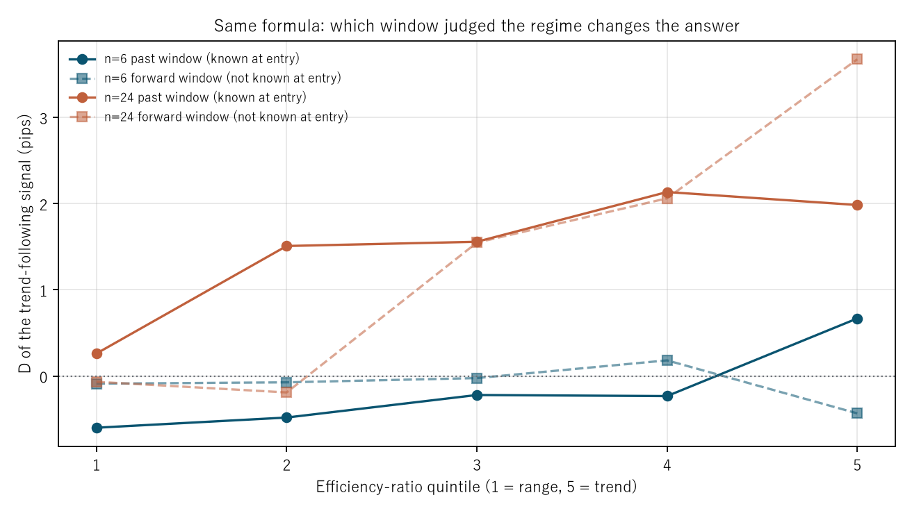
Figure 1: horizontal is the efficiency-ratio quintile, vertical is D of trend-following. Solid lines are the past window, dashed lines the forward one.
4. Judging the regime on the forward window
Calculation 4.1 Past window against forward window (D, pips)
| Window | Layer | Past D | Look-ahead D | Ratio |
|---|---|---|---|---|
| 6 | 1 | −0.5990 | −0.0882 | 0.15 |
| 6 | 3 | −0.2195 | −0.0233 | 0.11 |
| 6 | 5 | 0.6684 | −0.4326 | −0.65 |
| 24 | 1 | 0.2614 | −0.0666 | −0.25 |
| 24 | 2 | 1.5086 | −0.1898 | −0.13 |
| 24 | 3 | 1.5576 | 1.5478 | 0.99 |
| 24 | 4 | 2.1346 | 2.0616 | 0.97 |
| 24 | 5 | 1.9839 | 3.6741 | 1.85 |
Observation 4.2: The end-to-end spread goes from 1.7225 to 3.7407 pips at n=24, a factor of 2.2. But at n=6 it narrows from 1.2673 to 0.3444 pips, a factor of 0.3.
Observation 4.3: Prediction ① therefore holds only at n=24. ★ "Add look-ahead and anything gets bigger" is not true.
Observation 4.4: ★ The reason is that the efficiency ratio is a magnitude. Built from absolute values, it says how straight the move was, not which way. So only magnitude leaks.
Observation 4.5: ★ This is the same structure as F007. A quantity with no direction cannot call a direction, however much of the future it knows.
Observation 4.6: At n=24, layers 3 and 4 give ratios of 0.99 and 0.97. ★ Almost identical values. The look-ahead bites only in the end layers.
5. Does a longer window leak more?
Calculation 5.1 Window length and multiple
| Window | Past, end to end | Look-ahead, end to end | Multiple |
|---|---|---|---|
| 6 | 1.2673 | 0.3444 | 0.3 |
| 24 | 1.7225 | 3.7407 | 2.2 |
Observation 5.2: ★ Prediction ④ held. The multiple is 0.3 at n=6 and 2.2 at n=24 — the longer the window, the larger.
Observation 5.3: The largest daily |t| is 4.97 on the past window and 5.70 on the forward one. Adding look-ahead barely raises the t.
Observation 5.4: ★ So the after-the-fact step in the judgement window is smaller than expected. Where, then, does the apparent strength of "range → fade, trend → follow" come from?
Calculation 5.5 What comes out of taking whichever did better (★ added afterwards)
This is after the fact. Once it was clear that only magnitude leaks, another after-the-fact step was measured. Taking whichever of trend-following and counter-trend did better in each layer is just |D|.
| Window | Layer | Measured |D| past | Random |D| past | Measured |D| forward | Random |D| forward |
|---|---|---|---|---|---|
| 6 | 1 | 0.6020 | 0.3140 | 0.0882 | 0.0221 |
| 6 | 3 | 0.6275 | 0.1811 | 0.3133 | 0.1424 |
| 6 | 5 | 1.1636 | 0.5429 | 0.5996 | 0.7762 |
| 24 | 1 | 0.7824 | 0.1657 | 0.0888 | 0.1403 |
| 24 | 3 | 1.7671 | 1.1544 | 2.0001 | 0.8022 |
| 24 | 4 | 2.1346 | 2.0273 | 2.0616 | 1.0330 |
| 24 | 5 | 1.9839 | 1.0545 | 3.6741 | 1.6452 |
Observation 5.6: ★ This is the core. |D| is above zero in all 20 layers — on the measurement and on the synthetic random walk alike, without exception.
Observation 5.7: ★ The medians are 0.7050 on the measurement and 0.5544 pips on the random walk. Even on a series with zero directional information, taking whichever did better yields 0.5544 pips.
Observation 5.8: ★ So deciding the assignment "range → fade, trend → follow" from the results manufactures a number out of nothing. It bites far harder than the judgement window.
6. Baseline — do the same thing on a series with zero directional information
Calculation 6.1 Measurement against synthetic random walk (D, pips)
| Window | Layer | Past D | Look-ahead D | |
|---|---|---|---|---|
| 6 | 1 | measured | −0.5990 | −0.0882 |
| 6 | 1 | random | −0.3140 | 0.0012 |
| 6 | 5 | measured | 0.6684 | −0.4326 |
| 6 | 5 | random | −0.3297 | −0.2035 |
| 24 | 1 | measured | 0.2614 | −0.0666 |
| 24 | 1 | random | −0.1657 | 0.1064 |
| 24 | 3 | measured | 1.5576 | 1.5478 |
| 24 | 3 | random | −1.1544 | 0.8022 |
| 24 | 5 | measured | 1.9839 | 3.6741 |
| 24 | 5 | random | −0.3876 | −1.6452 |
Observation 6.2: Prediction ③ failed. The random walk's forward version has end-to-end spreads of −0.2048 (n=6) and −1.7516 pips (n=24), the opposite sign to the measurement's −0.3444 and +3.7407.
Observation 6.3: ★ The random walk's values are not small, however. At n=24 the forward version reaches −1.7516 pips. Even a series with zero directional information produces that much spread once it is cut into layers.
Observation 6.4: On the past window the random walk's end-to-end spreads are −0.0157 (n=6) and −0.2219 pips (n=24), far smaller. ★ Look-ahead makes a spread even on a random walk.
Observation 6.5: The largest daily |t| on the random walk's forward version is 5.98. Larger than the measurement's 5.70. The t value does not catch this error.
Observation 6.6: ★ So what the baseline says is that the sign of the look-ahead version cannot be trusted. If the same procedure produces the same magnitude with the opposite sign on a random walk, the measurement's sign is not a result of measuring.
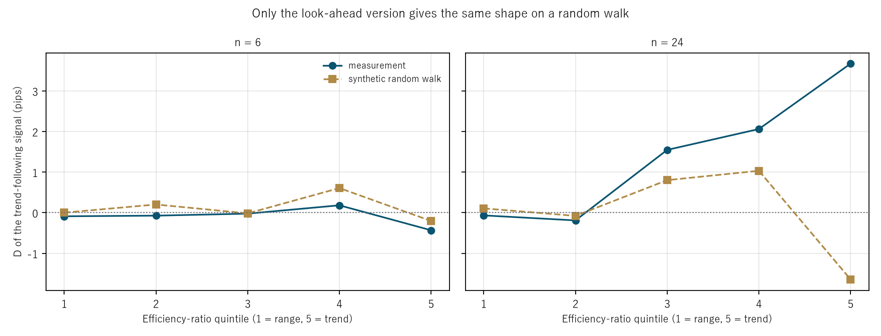
Figure 2: horizontal is the efficiency-ratio quintile, vertical is D under the forward window. The dark line is the measurement, the pale one the synthetic random walk.
7. Limitations
- ★ Predictions ② and ③ failed. The layer effect survives on the past window, and the random walk's forward version has the opposite sign to the measurement. This paper writes those failures.
- ★ Calculation 5.5 was added afterwards. It was measured once it became clear that only magnitude leaks, so it is after the fact.
- The layer cuts use the whole period. The quintile boundaries come from the whole sample, which is itself a mild look-ahead. Both versions are cut the same way, so the comparison is fair.
- The drift is not separated. That D is broadly positive at n=24 may be a statement about parts of these six years.
- The overlap is not removed. Measurements are taken on every bar, so the observations overlap.
- One definition of the regime is fixed. Other ways of measuring it give other figures.
- No costs are included. The figures here are therefore not trading performance.
- Four instruments over six years. Nothing is said about other markets or other periods.
Conclusion
"In a range you fade, in a trend you follow" has two places an after-the-fact step can enter: the judgement window and how the assignment is decided.
Switching the judgement window to the forward one widens the end-to-end spread across layers from 1.7225 to 3.7407 pips at n=24 (2.2 times). But at n=6 it narrows from 1.2673 to 0.3444 pips (0.3 times).
★ The reason is that the efficiency ratio is a magnitude. Built from absolute values, it says how straight the move was, not which way, so only magnitude leaks. This is the same structure as F007: a quantity with no direction cannot call a direction, however much of the future it knows.
Predictions ② and ③ failed. The layer effect survives on the past window (+1.2673, +1.7225 pips), and the random walk's forward version has the opposite sign to the measurement (−0.2048, −1.7516 against −0.3444, +3.7407).
★ So another after-the-fact step was measured (added afterwards). Taking whichever of trend-following and counter-trend did better in each layer is just |D|. It is above zero in all 20 layers, and even on a synthetic random walk with zero directional information the median is 0.5544 pips (against 0.7050 on the measurement).
★ What manufactures the number is not the judgement window but deciding the assignment afterwards.
And the daily t does not catch it. The largest daily |t| on the random walk's forward version is 5.98, larger than the measurement's 5.70. ★ What a report of "range → fade, trend → follow" needs is when that assignment was decided.
Data and reproduction
| Data | FX is Dukascopy-derived tick data (from 2019 onward, confirmed identical down to the millisecond, bid and ask). Gold is Dukascopy |
| Period | 2019–2024 (six years) |
| Instruments | USDJPY, EURUSD, GBPUSD, XAUUSD |
| Bars | One-hour bars, mid prices, closes of completed bars only. No bar is made where there are no ticks |
| Regime | Efficiency ratio = end-to-end ÷ path length, over the past n bars and over the next n bars |
| Window | n = 6 and 24 bars; layers are efficiency-ratio quintiles |
| Signal | Trend-following = sign(c[i] − c[i−n]); horizon is the change over the next n bars |
| Costs | Not included |
| Verification | 検算/F029.py (--zu also writes the figures). Every figure in the text comes from 検算/F029_output.txt |
| Figures | 図/F029_zu1, 図/F029_zu2 (png, svg, English versions) |
| Random seeds | Fixed. Re-running gives the same values |
| Foundation check | _ツール/audit_bars.py (bar look-ahead, daylight saving, day boundaries). The record is _土台の検査.txt |
References
- Yamagishi, Y. (2026). ADX Carries No Direction, So It Cannot Tell You Which Way [F007]. Zenodo. 10.5281/zenodo.22881623
Reference
Yamagishi, Y. (2026). Look-Ahead Leaks Only Magnitude; What Manufactures a Number Is Deciding the Assignment Afterwards [F029]. Zenodo.
DOI: 10.5281/zenodo.22893385
YOI: https://www.yamagishiyuuki.com/yoi/F029
ORCID: 0009-0006-8587-3450
PDF (English) · PDF (Japanese) · Date proof of the English PDF (OpenTimestamps .ots) · SHA256SUMS
The record page for this paper (in Japanese, with the PDFs in each language and the date proof): YOI F029. This paper is a preprint and has not been peer reviewed.