In an earlier article, “A Map of Inverse-Square Laws”, I drew a single map with the exponent of distance across and the dimension of space down. On that map there is a diagonal painted yellow. It is where the exponent equals the dimension exactly, and there a sum never stops growing.
“Could a theorem still be sleeping in the empty squares?” With that question in mind, I examined the yellow diagonal with numbers. What I found is that the never-ending sum splits cleanly into three parts. In this article I show what is inside, with figures and as few formulas as possible. The detailed calculations are in Paper 1098.
Add up the dots of graph paper inside a circle
Picture the dots of a sheet of graph paper (the points whose coordinates are whole numbers). Take the middle dot as the origin, and give every other dot a weight of “one over the distance squared”. Near dots weigh more and far dots weigh less: the same inverse-square weight as for gravity or the brightness of light.
Now add up this weight for the dots inside a circle of radius R.
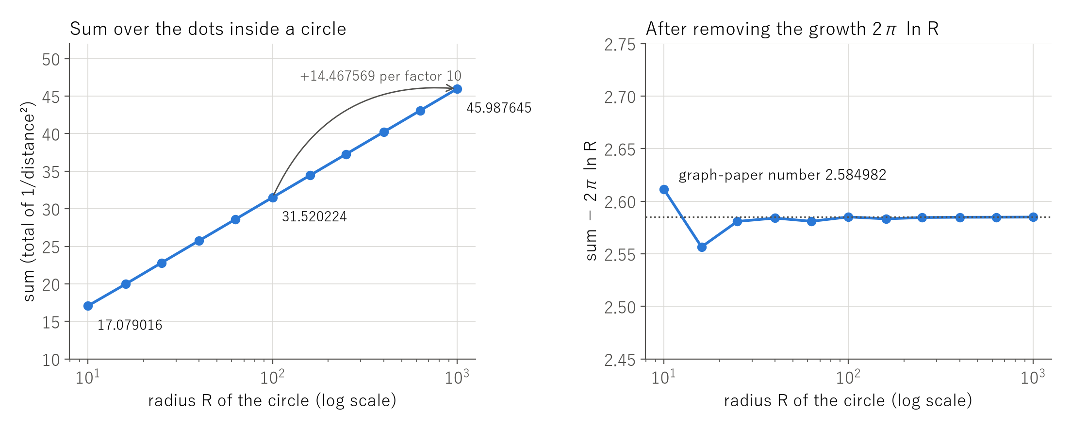
- Radius 10: 316 dots, sum 17.079016
- Radius 100: 31,416 dots, sum 31.520224
- Radius 1000: 3,141,548 dots, sum 45.987645
It is fun that the number of dots is almost π×R², but look at the sum. Each time the radius is multiplied by 10, the sum grows by about 14.467569. It never stops, yet it grows very slowly (mathematicians say it “grows logarithmically”).
Why it never stops: every ring adds the same
The reason becomes clear if we split the dots into rings: radius 1 to 2, 2 to 4, 4 to 8, doubling the radius each time we go outward. Outer rings hold more dots (8, 36, 148, 600: about 4 times as many each time), but each dot weighs less (twice the distance, so a quarter of the weight). The two effects cancel, and every ring adds almost the same amount to the sum.
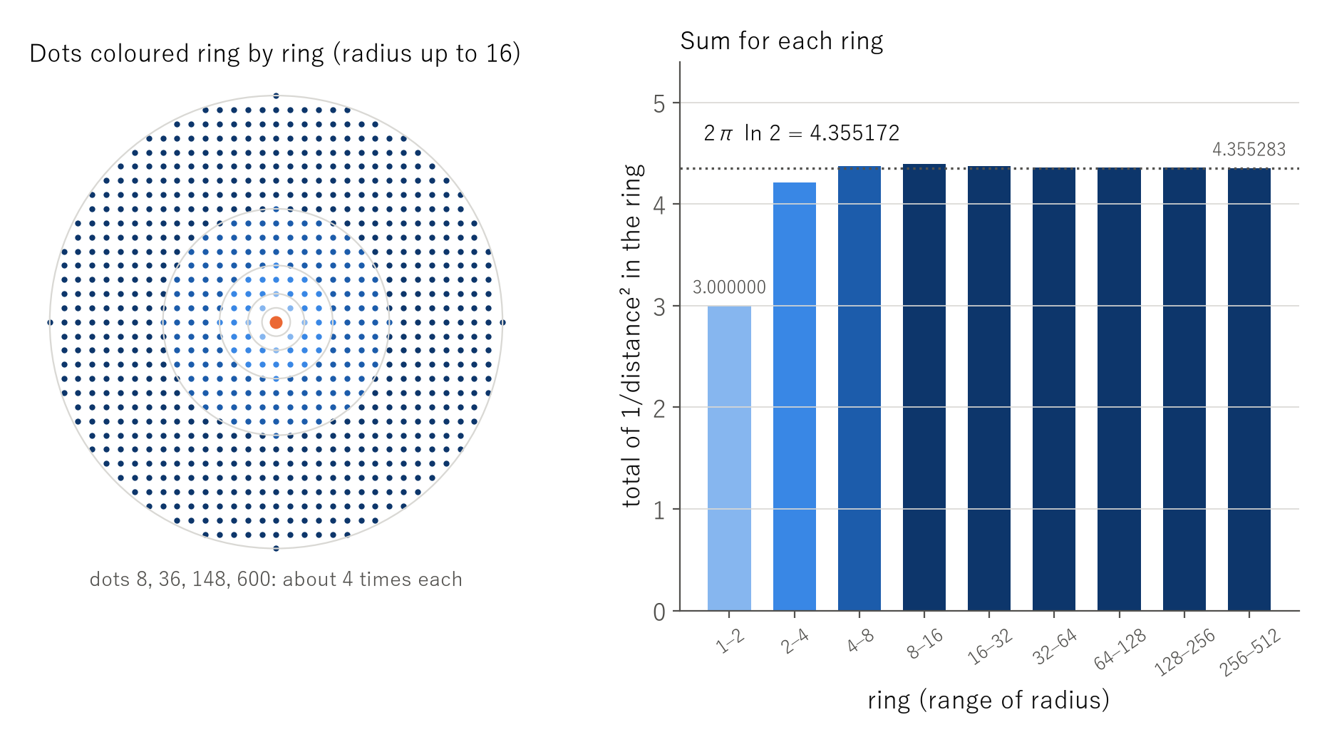
Rings that each add the same amount go on forever, so the sum never stops. This happens on a plane (two dimensions) with exponent 2, that is, only when the exponent equals the dimension. That is what the yellow diagonal of the map really is.
Remove the growth, and the “graph-paper number” remains
Since we know how the sum grows, we can subtract that growth (2π ln R). The sum then settles at a single number, 2.584982 (right side of Figure 1).
This number belongs to the lattice of the graph paper itself. It can in fact be written with a long-known formula (Kronecker’s limit formula), in which Euler’s constant γ and a special number, Γ(1/4), make an appearance. I will call it the “graph-paper number”.
Summed over a square, the answer is 0.691310 larger than over a circle
What if we sum over a square instead of a circle? Summing over a square with half side R and subtracting the growth in the same way, the answer came out 0.691310 larger than for the circle. Counting on the lattice, the difference had come down to 0.692372 at R = 3000. This 0.691310 has the form 2π ln 2 − 4G, where G is the number called Catalan’s constant (0.915966).
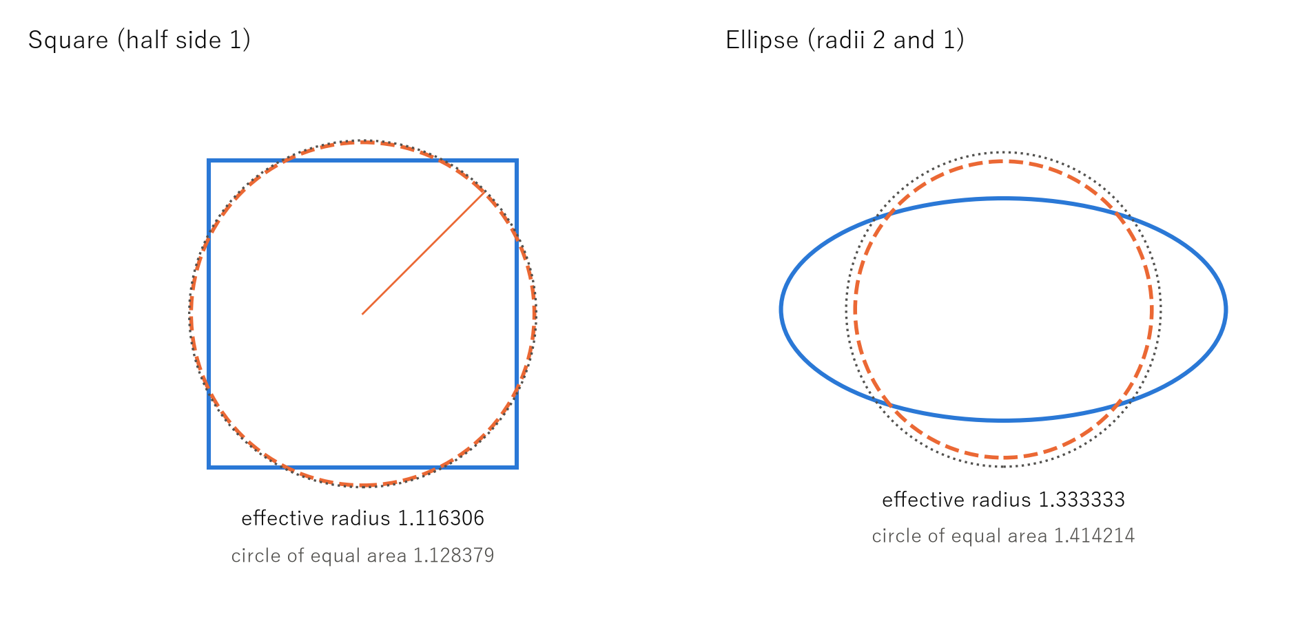
When I looked at where the shape enters, the answer was very simple. Measure the distance from the origin to the edge in every direction and take the average of its logarithm. That alone decides the effect of the shape. In other words, for large R, summing over any shape is the same as summing over a circle whose radius is the geometric mean of the distance to the edge. I call it the “effective radius”.
- The effective radius of a square (half side 1) is 1.116306, slightly smaller than 1.128379, the radius of the circle of equal area.
- The effective radius of an ellipse (radii 2 and 1) is 1.333333, exactly the harmonic mean of the two radii, 2×2×1÷(2+1) = 4/3. The circle of equal area has radius 1.414214.
For the same size, the circle (ball) wins
The effective radius is always at most the radius of the circle or ball with the same area (volume). It is equal only for a circle or ball centred at the origin. This follows at once from a relation known in mathematics as Jensen’s inequality.
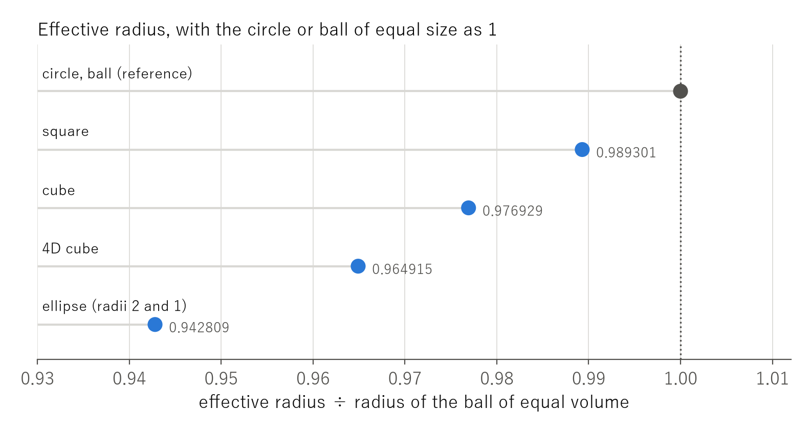
It is the intuition that taking the heavy, near dots first gives the most, turned directly into a number. I also checked it by actually summing lattice points for the cube and the four-dimensional cube (they approach shape numbers of 2.416955 and 5.099693).
Change the graph paper to triangles, and the shape number stays
Next, let us change the lattice itself: the arrangement you get when you pack coins flat as tightly as possible (the triangular lattice), with the same density of dots as the graph paper.
The number playing the role of the graph-paper number then changed to 2.518477 (0.066504 smaller than for graph paper). But the difference between square and circle, 0.691593 at R = 1000, approaches the same 0.691310 as on graph paper.
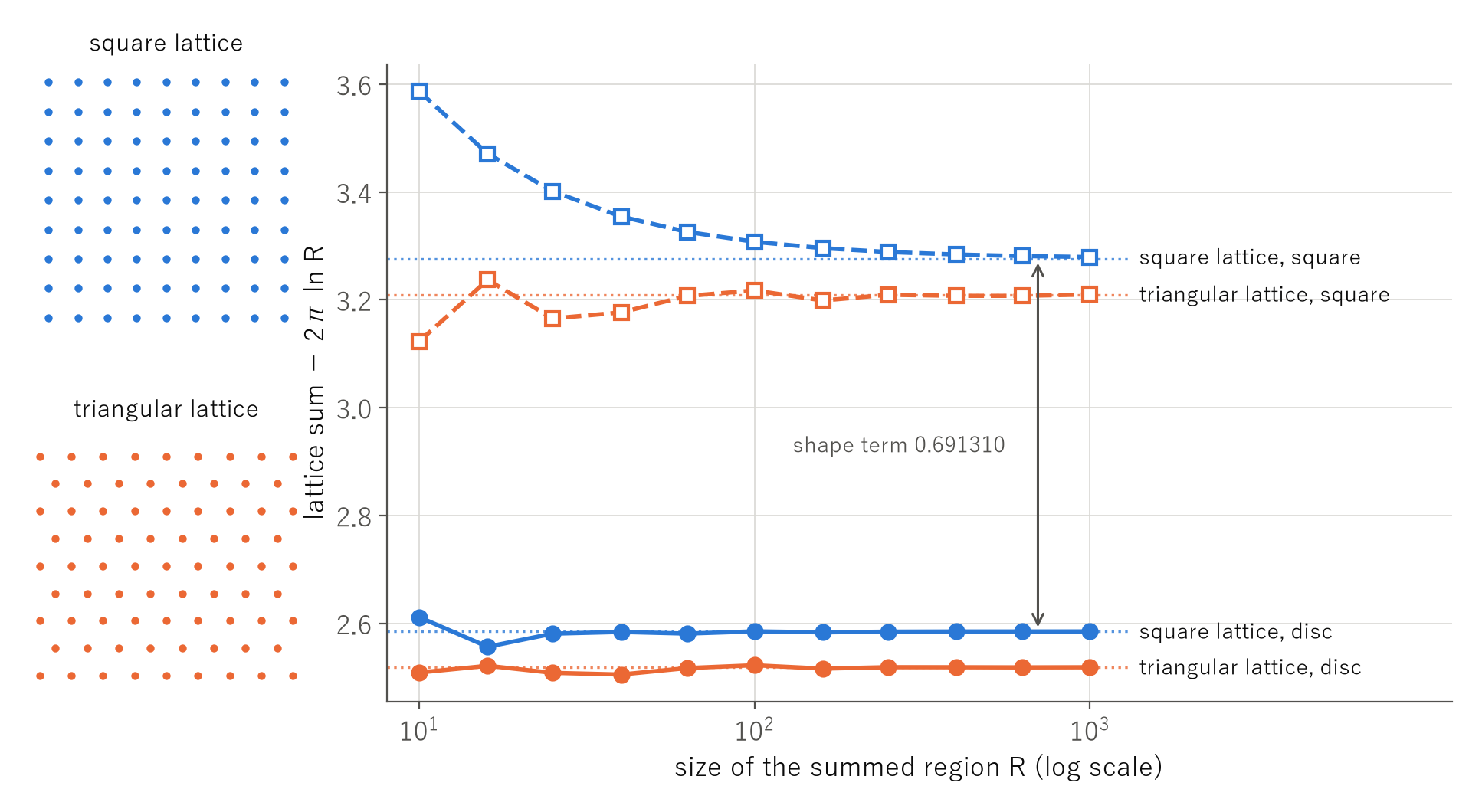
The shape number does not know the lattice, and the lattice number does not know the shape. The three parts did not mix. In the number of the triangular lattice, a different special number, Γ(1/3), appears in place of the Γ(1/4) of graph paper.
Change the dimension, and the lattice number shows a new face
I did the same from one dimension up to eight (with the weight “one over the distance to the power of the dimension”). The lattice number shows a different face in each dimension.
- One dimension: 2γ = 1.154431, made of Euler’s constant alone. This is the harmonic series, the same place as Paper 435 on Zipf’s law.
- Two dimensions: 2.584982, with Γ(1/4).
- Four dimensions: 4.632326, with Glaisher’s constant A (1.282427).
- Six dimensions: 5.677514, with β′(3) and ζ(3).
- Eight dimensions: 8.337340, where the ln 2 inside the formula cancels exactly.
- Three, five and seven dimensions: 3.821924, 5.131696 and 6.662093. Along the route used here they did not close into formulas and came out as numbers only.
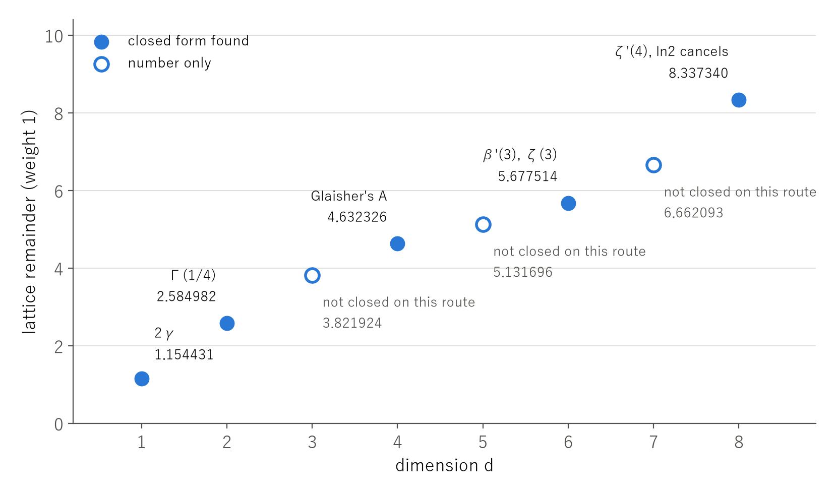
The number of the three dimensions we live in, 3.821924, was on the side that does not close along this route. Whether it closes along another route I have not checked. The closing dimensions 1, 2, 4, 6, 8 also look like the famous 1, 2, 4, 8 of numbers (real numbers, complex numbers, quaternions, octonions), but differ in having a 6. My rule is not to call two things the same root just because their sequences look alike.
With the weight of a magnet’s direction, only the shape number remains
So far every direction got the same weight. Now let us give a plus weight along the axis and a minus weight sideways, like the direction of a bar magnet (the dipole weight). Averaged all the way around, this weight is exactly 0.
Then the never-ending growth disappears. The graph-paper number also becomes 0, because plus and minus cancel ring by ring. Only the shape number remains, and it turned out to be exactly the quantity physics calls the “depolarization factor” (or demagnetizing factor).
- Summed over a sphere: 0
- Summed over a thin needle: 4π/3 = 4.188790
- Summed over a thin plate: −8π/3 = −8.377580
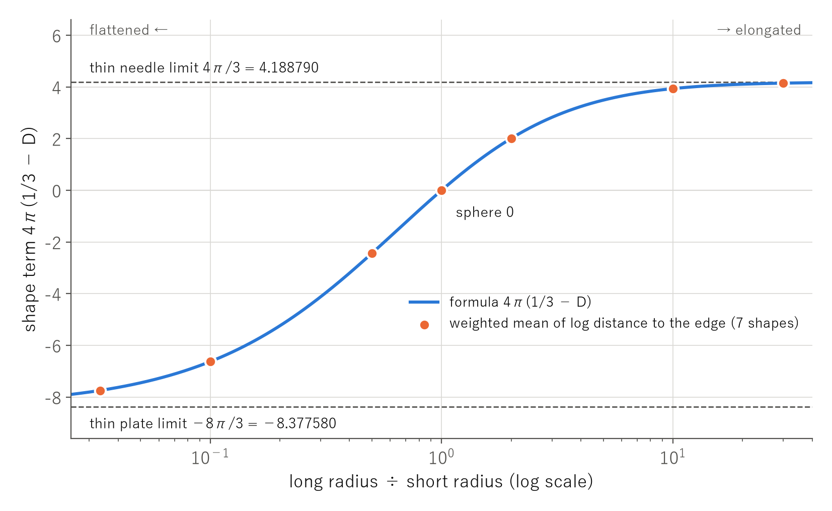
The depolarization factor tells how much the field inside a magnet or a dielectric is weakened by its shape, and textbooks compute it with integrals over ellipsoids. It can now be written in one line as “the average of the logarithm of the distance to the edge, weighted by the magnet’s direction”. In the earlier Paper 1097 I counted that a sum of dipoles placed on a lattice gives 0 for a sphere, 4π/3 for a needle and −8π/3 for a plate; those numbers came from this shape number alone.
When the lattice’s turns match the weight’s turns, something remains
Finally, I tried a weight with a finer pattern: one with four peaks of plus and four troughs of minus around the circle (cos4θ). It also averages to 0, so there is no never-ending growth.
On graph paper, however, the rings did not cancel, and the sum settled at 2.507655. On the triangular lattice every ring cancelled exactly, giving 0. For a weight with six peaks and six troughs (cos6θ) it was the other way round: 4.501541 remained on the triangular lattice.
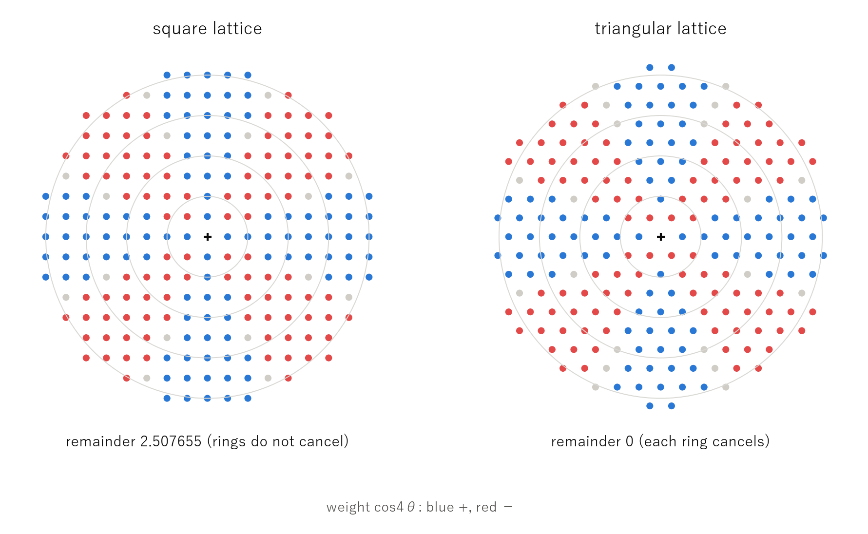
Graph paper returns to itself after a turn of 90 degrees, and the triangular lattice after a turn of 60 degrees. Only when the pattern of the weight is unchanged by turning the lattice does a sum remain. Computing the remaining numbers to high precision and feeding them to a tool that searches for relations between numbers, I found that the 2.507655 of graph paper matches Γ(1/4)⁸/(384π³) (ϖ⁴/(6π) with the lemniscate constant ϖ), and the 4.501541 of the triangular lattice matches √3Γ(1/3)¹⁸/(2048π⁸), to more than 40 digits (I have not proved them). Here too, Γ(1/4) appears for graph paper and Γ(1/3) for the triangular lattice.
Summary: the three parts of a never-ending sum
The sum on the yellow diagonal split into three parts.
| Part | What decides it | Example |
|---|---|---|
| Never-ending growth | the weight averaged around the circle (gone if the average is 0) | on graph paper, +14.467569 per factor 10 in radius |
| Lattice number | the lattice and the dimension (not the shape) | graph paper 2.584982, triangular lattice 2.518477, three dimensions 3.821924 |
| Shape number | the average logarithm of the distance to the edge (not the lattice) | square 0.691310; for the magnet’s weight, the depolarization factor |
There were two things whose change turns one case into another (I call them separators). Whether the weight averages to 0 around the circle decides whether there is never-ending growth. Whether turning the lattice cancels the weight ring by ring decides whether a lattice number remains. The shape number always remains.
About this article
This article does not claim any new law. The tools I used, such as the Epstein zeta function, Kronecker’s limit formula and the depolarization factor, are all long known. What I did was to line them up on the yellow diagonal of the map of inverse-square laws, split the sum into three parts, and check the numbers from one dimension to eight. Every number comes from the check scripts of the papers. All of the papers are preprints that have not been peer reviewed (the pages are in Japanese, with the paper PDFs in Japanese and English).
- Paper 1098: In a Lattice Sum Whose Exponent Equals the Dimension, Shape Enters as the Mean Logarithm of the Distance to the Edge
- Paper 1097: A Lattice Sum of Dipole Fields Is Decided by the Shape of the Summation: 0 for a Sphere, 4π/3 for a Thin Needle, −8π/3 for a Thin Plate
- Paper 1094: The “Squared Distance” in Retail Gravity Models Is, on a Map, the Exponent at the Border Where the Total Number of Customers Stops Converging
- Paper 435: Constant at Every Rank, and the Total Is Still Undetermined
- Paper 230: There Are Seven Minus Signs, and One of Them Undoes No Addition
- Paper 01: The Uniqueness Theorem of n = 2 for Spherically Symmetric Density Distributions
The whole map is in the earlier article, “A Map of Inverse-Square Laws”.