In the previous article, “Rearrange the Inside of a Box and the Gravity Outside Does Not Change at All”, I wrote that from outside a closed skin one can read only one number per angular pattern, one skin’s worth of pattern. Yet there are techniques that image the inside from outside. Hospital ultrasound is one. Kenjiro Kimura and colleagues at Kobe University have built a theory that measures while moving both the point that sends a wave and the point that receives it, and they are developing microwave mammography, which images the inside of the breast with radio waves.
I deeply respect Professor Kimura’s way of thinking. I once wrote on note that what I learned from my fishing master, learning the times when nothing bites, looks like the same shape as Professor Kimura’s inverse problem. This time I checked the part of that shared shape that can be said by calculation. What must be added to read an inside that cannot be read from outside? The answer was: move the frequency, or add a second point.
The calculations here were made new for this page, or come from the author’s own papers, released as preprints that have not been peer reviewed.
Key points
- Measured by receiving only, with no point that sends, whether the field is static like gravity or a wave of one frequency, what goes outside is one number per angular pattern. A rearrangement invisible from outside always exists, in a form tuned to that frequency.
- The form of the invisible rearrangement changes with the frequency. Move the frequency, and no rearrangement stays invisible at every frequency.
- Moving the frequency over a band, or measuring with two points that send and receive, the number that can be read grows gradually. For a spherically symmetric inside, two points at one frequency read about as much as receiving only with the frequency moved up to twice as high.
- The scattering-field equation of Professor Kimura and colleagues describes only how the outgoing and returning waves travel through an empty region, and for a single bounce it holds without approximation. The image stands only where the premise of that equation, an empty region, breaks down, that is, at the scatterers.
- Receiving only
- Invisible rearrangements
- Moving the frequency
- A second point
- Kimura’s equation
- The quiet of fishing
- Two roles of 1/r²
- Questions
- References
Receiving only, one per pattern at every frequency
Let the inside lie in a ball of radius 1. The field measured outside is either static, like gravity or electricity, or a wave, like sound or light. Waves are treated one frequency at a time. “Receiving only” here means that the field produced by the inside may be measured anywhere outside, as often as we like, but there is no point that sends.
With this kind of measurement, what goes outside is only one number per angular pattern. The field weakens as the outside radius changes, but the way it weakens is a fixed shape set by the pattern and the frequency, and it carries no details of the inside. I divided the inside into 40 layers along the radius and built the field at 30 outside radii by numerical integration, without using the expansion formula. In 16 cases, static and frequencies 2, 5 and 10, patterns 0 to 3, the second singular value was at most 2.24×10⁻¹⁴ of the largest. In every case, one number goes out. That it is one at a single frequency was also counted for the Helmholtz kernel in Paper 1107.
What reaches far away at one frequency is the inside split into components by fineness (its Fourier transform), read on the sphere of radius k. One may call it one skin’s worth in Fourier space. Gravity is the case of frequency 0, where that skin shrinks to a single point at the centre.
The invisible rearrangement moves with the frequency
In the previous article we checked that rearranging the inside of a box in the form Δφ (the curvature of a smooth hill φ) does not change the gravity outside. The same happens for waves. For a wave of frequency k0, a rearrangement of the form (Δ + k0²)φ sends nothing out. The Δφ of gravity is the case k0 = 0.
But measured at another frequency, the same rearrangement does come out. What goes out carries a weight of (k0² − k²). Move the frequency k0 to which the rearrangement is tuned, and the frequency k at which it is measured, in the figure below.
The upper slider chooses the frequency k0 the rearrangement is tuned to; the lower slider chooses the measured frequency k.
- number sent out at this frequency
- number sent out at the tuned frequency
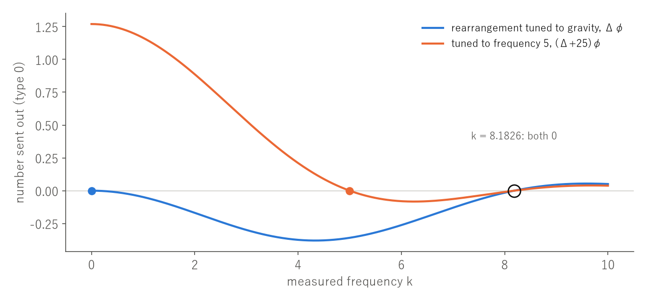
In numbers: the rearrangement tuned to k0 = 5, (Δ + 25)φ, sent out 1.2698413, 0.8870017, −0.0000000 and −0.0095429 at frequencies 0, 2, 5 and 8. The Δφ tuned to gravity sent out −0.0000000, −0.1689527, −0.3590739 and −0.0156601. Each is zero only at the frequency it is tuned to, and comes out elsewhere.
The invisible frequency need not be single, though. At a frequency where φ itself sends nothing out (k = 8.182561 for this φ), both rearrangements become invisible (Figure 1). If one measures only at finitely many frequencies k1, k2, …, a rearrangement of the multiplied form (Δ + k1²)(Δ + k2²)…ψ stays invisible at all of them. Even so, once the frequency is moved over a band, the only rearrangement invisible at every frequency is zero. What goes out is the value of the Fourier transform on a sphere; moving over a band reveals it on a whole thick spherical shell, and if the inside lies only within the ball, being zero there means being zero everywhere.
Moving the frequency, the numbers grow gradually
Still receiving only, move the frequency over a band. I measured at 400 frequencies from 0.05 up to the top k_max, divided the pattern-0 inside into 60 layers, and counted the numbers that can be read with singular values.
The slider moves the top of the band k_max. The buttons change the counting line (the size of the noise).
- numbers above the line
- k_max/π
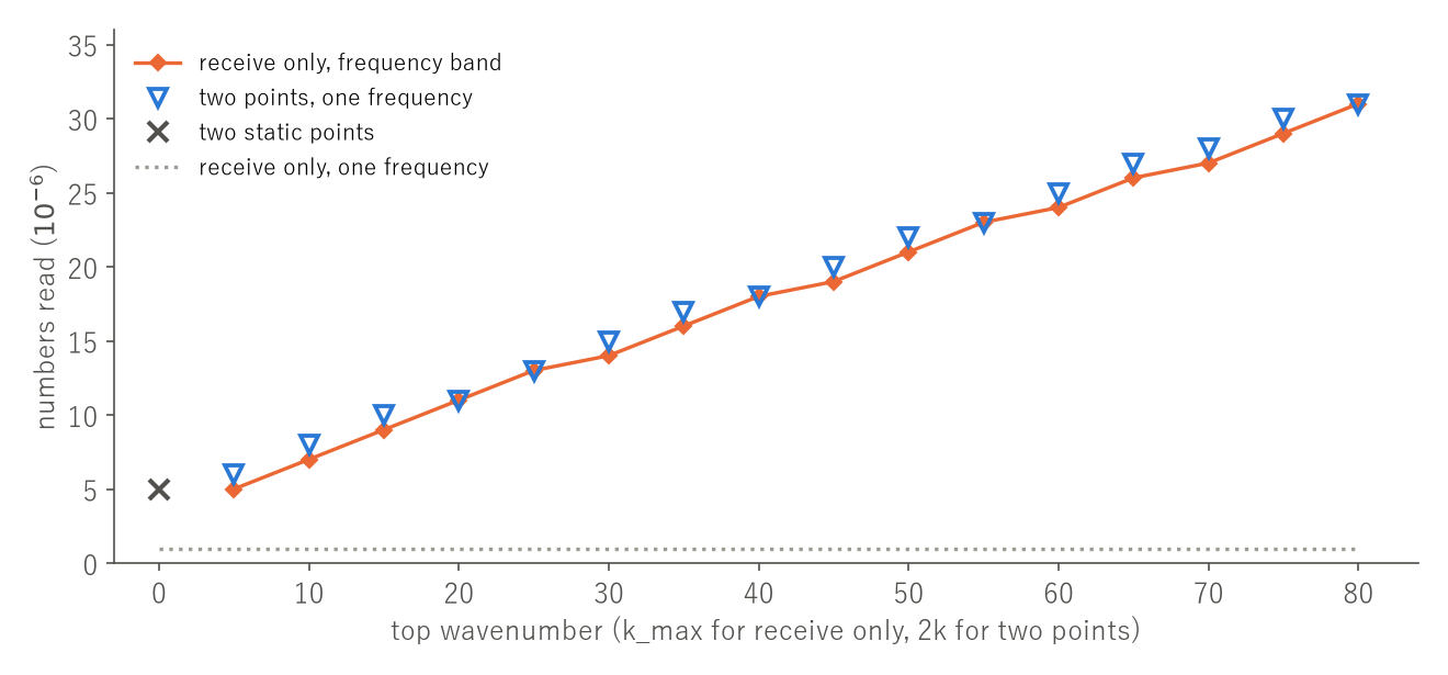
The numbers above 10⁻⁶ of the largest were 5, 7, 11, 18 and 31 for tops 5, 10, 20, 40 and 80. They grow by about one each time the top grows by π; k_max/π is the number of half wavelengths that fit in the radius 1. Unlike the cliff of a single frequency, the singular values thin out gradually. Where to cut is set by the size of the noise.
Adding a second point
Now keep one frequency, and move two points, the one that sends and the one that receives, on a skin of radius 1.5. The inside bounces the wave only once, and the strength of the bounce is put in a spherically symmetric (pattern-0) density. Receiving only at one frequency reads a single number for pattern 0, but two points read many layers.
The slider moves the frequency k. The buttons change the counting line.
- two points, one frequency
- receive only, band [0.05, 2k]
At the line 10⁻⁶, two points at frequencies 5, 10 and 20 read 8, 11 and 18, nearly the 7, 11 and 18 read by receiving only over the bands [0.05, 10], [0.05, 20] and [0.05, 40]. There and back, the fineness that can be read reaches 2k. This is the same count as diffraction tomography (Wolf 1969), which reads the inside up to the sphere of radius 2k by moving the direction of the incoming plane wave and the direction in which it is received far away. Stopping the frequency, two static points still read 5, but their singular values fall fast, a reading weak against noise. This is the side of the Calderón problem, reading the inside with electrodes on the body (Paper 99).
Professor Kimura’s equation is an equation of the empty region
Professor Kimura and colleagues wrote the scattering field as a function of two points, the one that sends and the one that receives, and derived the equation it satisfies (Kimura and Kimura 2021). For one scattering point, a spherical wave from the sending point to that point is multiplied by a spherical wave from that point to the receiving point and by the strength of the bounce, and this is summed over all scattering points. The two points share one coordinate x. In RIMS Kokyuroku, this equation (equation (2-5)) is derived as an approximation that drops higher terms in the inverse distance. With the values on the measured surface as boundary conditions, the equation is solved inwards in the space of two points; bringing the two points to the same point and summing over frequencies (returning the time to zero) gives the image.
When I checked, the equation held without approximation for a single bounce. The reason is short. The outgoing wave and the returning wave each travel freely through an empty region, and each satisfies its own wave equation. Splitting the shared x into two and putting those two equations into the operator, the fineness in the transverse direction (the wavenumber) cancels exactly, and the whole expression becomes zero. Computed at 40 digits, the remainder was below 10⁻⁴¹ of the size of the terms; for comparison, a product with the frequency of the return alone multiplied by 1.3 gave 0.148 and 0.181, and a product of static waves gave 1.000 and 0.272, not zero. Building the image on a wave equation that holds at each of the sending and receiving points is the same idea as the double-square-root equation of seismic exploration, which sinks the sending and receiving points together (Yilmaz and Claerbout 1980; Claerbout 1985).
The approximation actually works at the next step, where the depths of the sending and receiving points are aligned to the one measured surface. There, the point is chosen where the outgoing and returning waves travel in the same direction (a point of stationary phase). The European patent application on the same theory uses the words “almost an exact solution”, but that sentence is about another arrangement, in which the two points share two coordinates, x and the depth z. What I checked is equation (2-5), where only x is shared. I have not checked whether Professor Kimura and colleagues wrote this exactness in other papers. I read three: the paper in RIMS Kokyuroku, the paper on ultrasound, and the patent application.
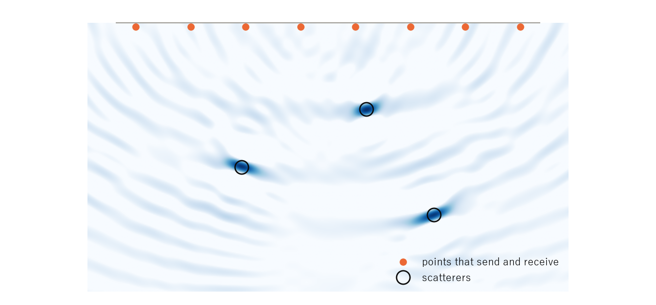
This equation contains not a trace of the strength of the scatterers. It describes only the outgoing and returning waves travelling through an empty region; one might call it an equation of the empty region. That is why it can be solved inwards with only the measured values as boundary conditions. The clue to the scatterers enters only through the measured signals (the boundary values). When the equation is solved inwards, the two points are brought to the same point and the time returns to zero, values stand only where the points that send and receive meet a scatterer, that is, only where the premise of the equation, an empty region, breaks down. The figure below is a very simple two-dimensional sample for seeing this idea. It is not the computation of Professor Kimura and colleagues itself.
The slider changes how many points are lined up on the top line. Any two of them serve as the point that sends and the point that receives.
- pairs used
With one pair, the arrival time of an echo tells only the set of points whose echoes arrive at that time: a circle if the sending and receiving points coincide, an ellipse if they are apart. Adding pairs, the circles and ellipses overlap only at the scatterers, and peaks stand there. Placing the image where downgoing and upgoing waves meet in time and place has long been used in seismic exploration too (Claerbout 1971).
In the ideal limit where all frequencies are present, the image of a point scatterer is sharp at one point, and its value does not stay finite. With a real band, the width of the peak is set by the bandwidth. For the band [π, 2π] (frequencies 0.5 to 1) the first zero of the envelope is at 1.000000, the same formula as the radar range resolution c/2B (Paper 802).
The quiet of fishing, and an equation of the empty region
My fishing master did not only look for bites; he drilled into his body the state when nothing was biting. On note I wrote that this looks like the same shape as Professor Kimura’s inverse problem: that Professor Kimura defined a quiet, empty space as an equation and looked for the places where that quiet breaks. In Paper 89 I kept this connection outside the calculations, as a personal impression rather than science.
This time part of it can be said in numbers. The equation of Professor Kimura and colleagues truly describes only how waves travel through an empty region, and the scatterers emerge as the points where the premise of that equation, an empty region, breaks down. Where I wrote on note about “the points where the values diverge”, in the ideal limit with all frequencies the image of a point is sharp at one point, so in that sense it was right. With a real band it becomes a peak whose width is set by the bandwidth. The fishing technique itself I still keep outside science.
Two roles of 1/r²
The 1/r² of gravity and electricity is a field with no source outside the inside. The flux through any closed surface is 4π times the amount inside, whatever the shape of the surface and wherever the inside lies. This 4π comes from the field being massless. That what goes outside is one number per angular pattern has a different root: the field equation is of second order and local (Paper 1107; the massive Yukawa field, too, sends out one number per pattern). In this sense the 1/r² field, as the representative of second-order fields, hides the inside from outside.
For waves, the same 1/r² plays another role. That the flow of an outgoing spherical wave does not depend on the radius fixes its amplitude at 1/r, and in three dimensions an echo arrives, weakening, without changing its shape. The next article, “Only in Three Dimensions Does an Echo Come Back with Its Shape Unchanged”, checks this. Still, what lets the method of Professor Kimura and colleagues read the inside is not so much that the echo keeps its shape as that what two points, one sending and one receiving, measure does not fit into one function on the skin.
Questions
Can gravity alone not reveal everything inside the Earth?
Gravity alone reveals only one number per angular pattern. Adding waves with frequencies, like seismic waves, or methods that change the sending and receiving points, increases what can be known about the inside.
With two points, is every inside determined uniquely?
The calculations on this page use an inside that bounces the wave once (the Born approximation) and look only at the pattern-0 density. Whether it is determined uniquely and whether it can be read robustly against noise are different questions, and the number that can be read moves with the counting line (the size of the noise).
Is the method of Professor Kimura and colleagues an approximation?
In RIMS Kokyuroku the equation was derived as an approximation, but for the formula of a single bounce it held without approximation. The approximation works at the step where the depths of the two points are aligned to form the image. Waves that bounce many times, or media whose properties change with frequency, are not treated on this page.
Papers and references
All papers are published under CC BY 4.0.
- Paper 1111 “The Inverse Square Hides the Interior from a Static Field and Carries the Echo of a Wave Undistorted”: the source of the calculations on this page.
- Paper 1107 “When the Field Equation Is of Second Order, the Interior Can Be Read from Outside a Closed Skin Only as One Number per Angular Pattern”: the count when receiving only.
- Paper 89 “Zero-Tension and the Inverse Problem”: the connection between fishing and inverse problems.
- Paper 99 “Reading the Interior from the Boundary”: the Calderón problem.
- Paper 802 “Radar Range Resolution Comes from Bandwidth, Velocity Resolution from Time, and a One-Wrap Velocity Error Shifts Range One Cell”: the range resolution c/2B.
- Kimura, K., and Kimura, N. (2021). Inverse Scattering filed theory [title as printed]. RIMS Kokyuroku, Kyoto University.
- Yabumoto, K., Yumii, T., and Kimura, K. (2025). Research on Ultrasonic Imaging Systems Based on Scattering Field Theory. arXiv:2508.14469.
- Kimura, K., Kimura, N., and Kimura, F. (2024). Video-forming device and video-forming method. European Patent Application EP 4357766 A1.
- Wolf, E. (1969). Three-dimensional structure determination of semi-transparent objects from holographic data. Optics Communications.
- Claerbout, J. F. (1971). Toward a unified theory of reflector mapping. Geophysics.
- Yilmaz, Ö., and Claerbout, J. F. (1980). Prestack partial migration. Geophysics.
- Claerbout, J. F. (1985). Imaging the Earth's Interior. Blackwell Scientific Publications.